Author: Aloe Labs, Inc
This Uniswap simulator is designed to make it easier to analyze and develop new liquidity management strategies. It can handle everything from Uniswap v2 to arbitrary collections of v3 positions with dynamic fee compounding, rebalancing, and more. The only requirement is that the strategy be expressed as a series of operations on numpy arrays.
We recommend using our main script to run your strategy.
This will test it against 400 combinations of mu and sigma (Geometric Brownian
Motion parameters) and sample 1000 price trajectories for each combination.
To speed things up, operations are parallelized across CPU cores. The result is
4 files:
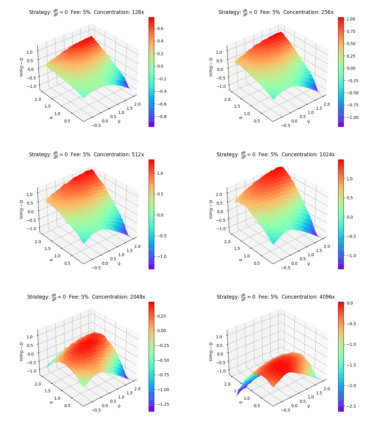
X.npyThe meshgrid of mu values (m x n)Y.npyThe meshgrid of sigma values (m x n)Z.npyThe asymptotic wealth growth rate of the strategy, and that of HODLing (m x n x 2)surf.pngA 3D plot ofZ[:,:,0] - Z[:,:,1], i.e. where z > 0 the strategy outperforms HODLing
We're using Poetry for dependency management. They've put together some really nice documentation here if you're unfamiliar. Once you have Poetry, install the simulator like so:
git pull https://github.com/aloelabs/uniswap-simulator.git
cd uniswap-simulator
poetry install
If this doesn't work, install Python 3.9 (
apt-get install python3.9 python3.9-dev) and try again.
There are many ways to use this library, but for now let's assume you just want to run one of our examples.
mkdir results
poetry run python examples/main.py
It may take up to 30 minutes to finish running, depending on your hardware. If you can't wait that long, decrease the mesh resolution on lines 43 and 44:
sigmas = np.linspace(0.1, 2.0, 20)  # change 20 to something lower (maybe 5)
mus = np.linspace(-0.8, 2.0, 20)  # same thing here
You will probably want to experiment with different strategies as well. You can change what's being simulated
by modifying lines 31-34. Two strategies have already been imported: a plain Uniswap v3 position (Position),
and one that's set to compound earned fees as quickly as possible (CompoundingStrategy):
# Setup the position's initial bounds. The denominator (2) indicates
# that it is twice as concentrated as a full-range position.
lower = np.full_like(prices[0], 1.0001 ** (MIN_TICK / 2))
upper = np.full_like(prices[0], 1.0001 ** (MAX_TICK / 2))

# Note that the fee tier is 5%. This is higher than current Uniswap pools allow,
# but necessary because of float precision issues in Python. It's okay because
# we're trying to compare strategies to one another, not perfectly predict
# real-world performance.
strategy = Position(prices[0], lower, upper, 5.00/100)
# strategy = CompoundingStrategy(prices[0], lower, upper, 5.0/100)
There are many other example strategies for you to import and try out. We divide them into two broad categories: dynamic and static. In static strategies, the largest Uniswap position is stationary over time. Earnings may be compounded into it, but its bounds don't change. In contrast, dynamic strategies allow the main Uniswap position to move -- usually they recenter it around the current price. Here's a list of strategies we've implemented:
- Position (built into the library) A plain Uniswap v3 position
- PositionV2 (built into the library) A plain Uniswap v2 position
- Compounding A Uniswap v3 position that compounds earnings into itself as often as possible
- Split Compounding A Uniswap v3 position that compounds earnings as often as possible. Splits main position into 2 (one fully denominated in token0, the other in token1) to compound fees when the fees0 : fees1 ratio wouldn't otherwise allow for perfect compounding
- dR/dP=0 A concentrated Uniswap v3 position that intelligently places earnings into range orders to maintain 50/50 inventory ratio. Both static and dynamic version available
