Flatiron Data Science Project - Phase 4

Prepared and Presented by: Melody Peterson
Presentation PDF
For this analysis I will be working as a Data Scientist for a financial investment firm that is looking for short-term real estate investment opportunities for it's smaller investors to diversify their investment profiles. I will be analyzing median monthly housing sales prices for over 14,000 United States zipcodes and choosing the best areas to further analyze for potential investment. I will then forecast future real estate prices in those zip codes.
There are many datasets available on the Zillow Research Page. The data used here represents median monthly housing sales prices for 14,723 zip codes over the period of April 1996 through April 2018 as reported by Zillow. Each row represents a unique zip code. Each record contains location info and median housing sales prices for each month. There are 14,723 rows and 272 variables: RegionID, RegionName (zip code), City, State, Metro, CountyName, SizeRank, finally 1996-04 through 2018-04 which represent 265 data points of monthly data for each zip code.
Starting with the initial data cleaning/scrubbing phase, it was discovered that many zip codes did not have the full date range of data. Some zip codes had data only going back to 06-2014. I chose not to eliminate any zip codes for missing values but would model on the data available. My next step was to calculate an ROI for each zip code that I could compare across all of the data, so for instance a 10 year ROI would not be possible. Since my business case was for short term investment opportunities, a 10 year ROI would not be necessary. I calculated a 4 year ROI and the most recent year (2018) ROI. Finally I calculated the average one year ROI over the past 3 years and chose to use that as my comparison metric.
Per my business problem, I was looking for the best ROI for small investors so I graphed ROI against the current Median Housing Price and then subset to the lower housing prices, eventually selecting six zip codes with high average ROI and low median housing prices for further analysis.
Here is a comparison of the data on the 6 zip codes over time. As you can see, Indianapolis and Columbus have limited data. But generally they all reflect the housing market crash of 2009 and then these six zipcodes have shown significant increases over the past 4 years.
This graph of the Philadelphia data shows how each time series can be broken out into trend, seasonality, and noise components.
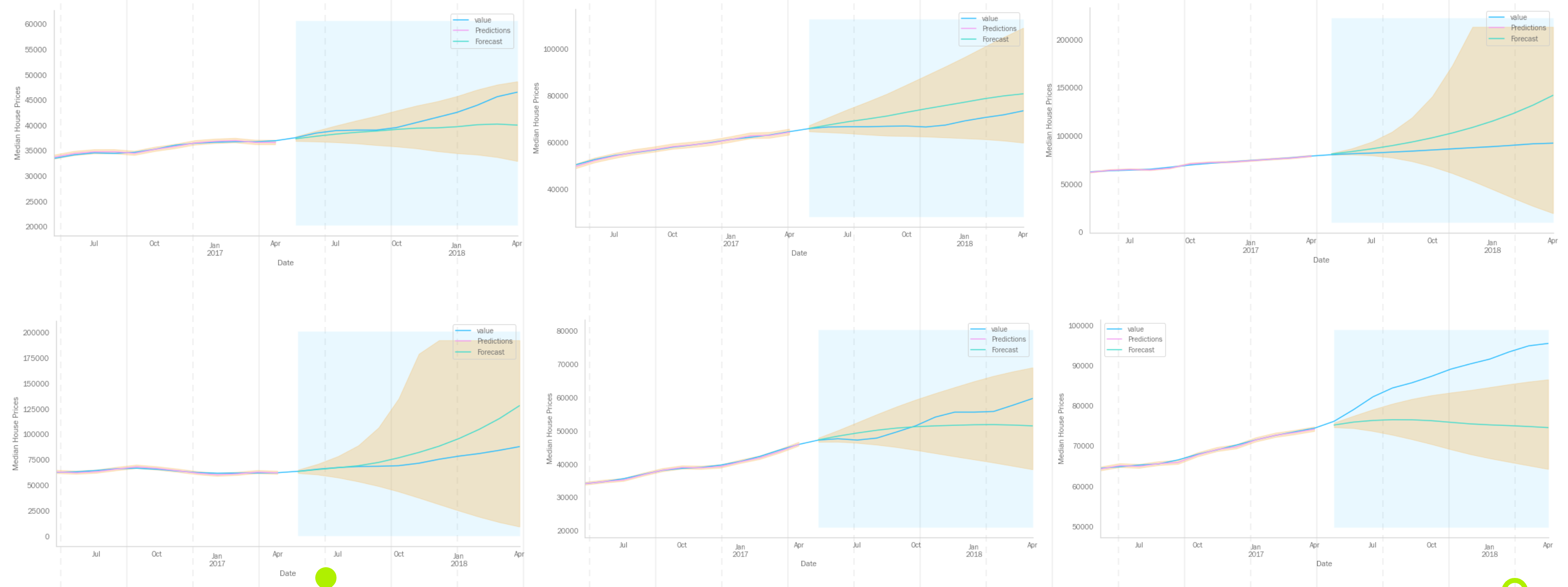
Initial ARMA (Auto-regressive Moving Average) models were run on all 6 zip codes to establish a baseline for future models, and then several models were run and parameters tuned to find the model with the least error.

Final Seasonal ARIMA model parameters
- All training data far outperformed the test data, indicating some overfitting.
- The models are all very skewed because of the market crash in 2009.
- Columbus and Daytona had very large confidence intervals and overly high forecasts.
- Chattanooga has outperformed even the confidence intervals of the model.
- Philadelphia is potentially a good 50K investment , Indianapolis at 75K and Chattanooga at 100K investment
- Logged and differenced the data but some still did not test as stationary according to the Dickey Fuller test.
- Real estate predictions can vary due to unseen fluctuations in the market
- Obtain current data after 2018 for current predictions. Found zip code data on Redfin but it is rolling avg by zip code.
- Investigate why some of the models seem so far off in their forecasts.
- Try Facebook Prophet with each of the chosen zip codes
- Try other methods of choosing zip codes, including clustering to find trends
- Look for exogenous data to add to the model


