autoOcc is an R package to fit an autologistic occupancy model, which is a simplified version of a dynamic occupancy model that is espcially useful when dealing with smaller datasets. autoOcc fits this model hierarchically so that different covariates can be used on a species latent occupancy and detection probability. Most of the functions here behave similarly to those in unmarked, so using autoOcc should be somewhat familar to those who have experience with that R package.
2023 - 07 - 18: Released version 0.1.1. There are two new features and two bug fixes.
- p values have been added to the estimates table for auto_occ_fit objects. As just one example here is a snippet from a summary of a
an
auto_occ_fitobject.
Occupancy estimates:

          parameter    Est    SE lower   upper        p
1 psi - (Intercept) -0.727 0.342 -1.40 -0.0574 0.033341
2  psi - Impervious -0.991 0.496 -1.96 -0.0187 0.045757
3       psi - theta  2.785 0.845  1.13  4.4403 0.000974
-
A new function,
autoOcc::model_list_estimates()to compile all the parameter estimates and standard errors from a list of models. This could be useful, for example, if you would like to do some model averaging. See the example analysis below to see this function be used. -
Added in some error catching in the event that duplicated site names were included within a primary sampling period within
autoOcc::format_y. Previously, this would error out in a non-informative way. -
There was a small bug with
autoOcc::predict().Previously, factors that did not use the standard ordering for levels (i.e., alphabetical) would get converted to alphabetical when making predictions. This would lead to wrong predictions. Factor level ordering is now retained.
This package is in active development. I'll likely just add in new functions when I locate some pain points while working with it. That said, the current functions are stable.
autoOcc can be installed from Github:
install.packages("devtools")
devtools::install_github(
  "mfidino/autoOcc",
  build_vignettes = TRUE
)
Mason Fidino is the sole contributing author of autoOcc, though some of the code used in this package was based on the code and analysis flow of unmarked.
If you are interested in contributing, see Contributor Guidelines.
If you want a more thorough walkthrough of a standard analysis in autoOcc,
and had made certain to build the vignettes when installing from github,
check out the overview vignette with:
vignette("Overview")library(autoOcc)
# load in the data
data("opossum_det_hist")
data("opossum_covariates")
# function to generate detection history
# for the opossum data, opossum_y is
# a site by primary sampling period by secondary
# sampling period array.
opossum_y <- autoOcc::format_y(
x = opossum_det_hist,
site_column = "Site",
time_column = "Season",
history_columns = "^Week" # start with Week
)
# scale the covariates for analysis
oc_scaled <- as.data.frame(
lapply(
opossum_covariates,
function(x){
if(is.numeric(x)){
scale(x)
}else{
x
}
}
)
)
# dropping site column from oc_scaled
oc_scaled <- oc_scaled[,-1]
m1 <- auto_occ(
~Impervious + Income ~ Impervious + Income,
y = opossum_y,
det_covs = oc_scaled,
occ_covs = oc_scaled
)
m2 <- auto_occ(
~Impervious~Impervious,
y = opossum_y,
det_covs = oc_scaled,
occ_covs = oc_scaled
)
m3 <- auto_occ(
~Income~Income,
y = opossum_y,
det_covs = oc_scaled,
occ_covs = oc_scaled
)
m4 <- auto_occ(
~1~1,
y = opossum_y,
det_covs = oc_scaled,
occ_covs = oc_scaled
)
# compare models, make a list object of the model first.
my_model_list <- list(m1, m2, m3, m4)
my_aic_results <- compare_models(
my_model_list,
digits = 2
)
# Compile all parameter estimates across models (could be helpful
# if you wanted to do model averaging).
all_estimates <- model_list_estimates(
my_model_list
)
round(all_estimates$estimates, 2)
# Looks like the first model, which included
# income and impervious cover, is the best
# fit model.
# model npar AIC delta AICwt cumltvWt
# 1 m1 7 1232.72 0.00 0.90 0.90
# 2 m3 5 1238.22 5.50 0.06 0.96
# 3 m4 3 1239.66 6.94 0.03 0.99
# 4 m2 5 1241.14 8.42 0.01 1.00
# Let's make predictions from this model.
# First, I make the prediction data.frame with a realistic
# range based on the actual data and not the scaled data.
# The range(oc$Impervious) is about 18 to 81, so choose 20
# to 80. We do this so that we have nice numbers for plotting.
# Likewise, we scaled all of the other data, so we leave Income
# at it's mean (i.e., 0) for predictions.
imperv_real <- data.frame(
Impervious = seq(20,80,0.5),
Income = 0
)
# We will use imperv_real for plotting purposes, but to make predictions
# we need to scale imperv_real$Impervious in the exact same way we did
# with the fitted model. Thus, we subtract the mean of the actual data
# and divide by the standard deviation.
imperv_scaled <- imperv_real
imperv_scaled$Impervious <- (
imperv_scaled$Impervious - mean(opossum_covariates$Impervious)
) / sd(opossum_covariates$Impervious)
# the model prediction across a gradient of Impervious cover
opo_imperv <- predict(
object = m1,
type = "psi",
newdata = imperv_scaled
)
# do the same thing with income
income_real <- data.frame(
Impervious = 0,
Income = seq(40000, 160000, by = 500)
)
income_scaled <- income_real
income_scaled$Income <-
(income_scaled$Income - mean(opossum_covariates$Income))/
sd(opossum_covariates$Income)
opo_income <- predict(
object = m1,
type = "psi",
newdata = income_scaled
)
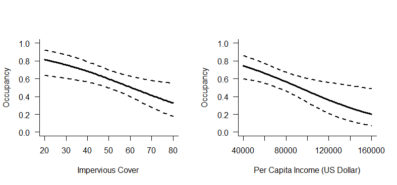
# plot them out
par(mfrow = c(1,2))
plot(
opo_imperv$estimate ~ imperv_real$Impervious,
bty = "l",
type = "l",
las = 1,
ylab = "Occupancy",
xlab= "Impervious Cover (%)",
ylim = c(0,1),
lwd = 3
)
lines(opo_imperv$lower ~ imperv_real$Impervious, lwd = 2, lty = 2)
lines(opo_imperv$upper ~ imperv_real$Impervious, lwd = 2, lty = 2)
plot(
opo_income$estimate ~ income_real$Income,
bty = "l",
type = "l",
las = 1,
ylab = "Occupancy",
xlab= "Per Capita Income (US Dollar)",
ylim = c(0,1),
lwd = 3
)
lines(opo_income$lower ~ income_real$Income, lwd = 2, lty = 2)
lines(opo_income$upper ~ income_real$Income, lwd = 2, lty = 2)

