Murray et al. (2021). A multi-state occupancy model to non-invasively monitor visible signs of wildlife health with camera traps that accounts for image quality. Journal of Animal Ecology.
This repository contains seven folders. In alphabetical order they are:
Contains two images used to make README.md. This includes:
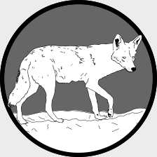
./assets/coyote.png: A line drawing of a coyote.
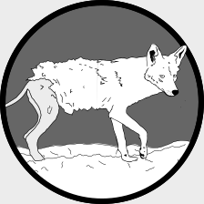
./assets/coyote_mange.png: A line drawing of a mangy coyote.
This folder contains the data to fit the model and a set of gridpoints as a shapefile used to generate figure 5 in the manuscript.
./data/coydata_merged_sites.csv: A csv file with 3971 rows and 11 columns that contains all of the image data used in the analysis.
| Column header | Data type | Description |
|---|---|---|
| new_file_name | character | The name of the coyote image, which generally uses a site code. |
| blur | numeric | The blur value calculated by the python script. Higher values indicate increased clarity. |
| File_name_order | integer | The numeric order of images at a site. |
| Mange_signs_present | boolean | Takes a value of 1 if mange was detected in an image, otherwise it is 0. |
| In_color | boolean | Takes a value of 1 if the image is in color, otherwise it is 0 (i.e., greyscale). |
| Season | categorical | The season the photo was collected. Either Spring, Summer, Fall, or Winter. |
| Year | integer | The year the photo was collected. |
| propbodyvis | proportion | The proportion a coyote was visible in an image, ranges from 0 to 0.55 |
| surveyid | character | The survey code for a photo. Combines seasonal, year, and site information. |
| site | character | The site the image occured at. |
| date | date | The date the image was taken |
coyote_detection_data.csv: A csv with 54656 rows and 8 columns that contains all of the coyote detection / non-detection data used in the analysis.
| Column header | Data type | Description |
|---|---|---|
| Season | categorical | A seasonal code for the season the data comes from. It combines the first two letters of the season and the last two digits of the year. Seasonal codes are SP = Spring, SU = Summer, FA = Fall, WI = Winter. Data collection started in 2010. |
| Week | categorical | The week of a given primary sampling period. Week 1 through Week 4. |
| Date | date | The date of the coyote detection / non-detection data. In yyyy/mm/dd format. |
| SeasonWeek | categorical | Just a combination of Season and Week columns. |
| StationID | categorical | The site code for the detection / non-detection data. Can be joined to the site column in coydata_merged_sites.csv |
| SurveyID | categorical | The survey code for the detection / non-detection data. Can be joined to the surveyid column in coydata_merged_sites.csv |
| IDWeek | categorical | Just a combination of the StationID and the Date |
| Coyote | Integer | Can take three values. NA if a camera was not active, 0 if the camera was active and coyote were not detected, and 1 if the camera was active and coyote were detected. |
./data/gridpoint.shp: A shapefile of the gridpoints used to predict coyote and coyote with mange throughout the greater Chicagoland area (figure 5). The utm coordinate
reference system for this file is 26916.
./data/map_data/coyote_mange_hu10.csv: The housing density calculated at
each of the gridpoints for figure 5. This csv is 28329 rows by 2 columns.
| Column header | Data type | Description |
|---|---|---|
| LocationName | integer | The site code from the gridpoints shapefile. |
| HU10 | numeric | The housing density (houses per km squared) in a 1 km buffer around each gridpoint. Data comes from http://silvis.forest.wisc.edu/data/housing-block-change/ |
./data/map_data/tree_imperv_mapdata.csv: The tree cover and impervious cover calculated at each of the gridpoints for figure 5. This csv is 28329 by 3 columns.
| Column header | Data type | Description |
|---|---|---|
| LocationName | integer | The site code from the gridpoints shapefile. |
| tree | percent | Percent tree cover in a 1 km buffer around each gridpoint. Data comes from https://datahub.cmap.illinois.gov/dataset/high-resolution-land-cover-ne-illinois-and-nw-indiana-2010 |
| imperv | percent | Percent impervious cover in a 1 km buffer around each gridpoint. Data comes from https://datahub.cmap.illinois.gov/dataset/high-resolution-land-cover-ne-illinois-and-nw-indiana-2010 |
./data/model_covariates.csv: The covariates used to generate the two
urbanization metrics via Principal Components Analysis. This csv has 113 rows and 4 columns.
| Column header | Data type | Description |
|---|---|---|
| site | categorical | The site code where data was collected. |
| house | numeric | The housing density (houses per km squared) in a 1 km buffer around each site. Data comes from http://silvis.forest.wisc.edu/data/housing-block-change/ |
| tree | percent | Percent tree cover in a 1 km buffer around each site. Data comes from https://datahub.cmap.illinois.gov/dataset/high-resolution-land-cover-ne-illinois-and-nw-indiana-2010 |
| imperv | percent | Percent impervious cover in a 1 km buffer around each site. Data comes from https://datahub.cmap.illinois.gov/dataset/high-resolution-land-cover-ne-illinois-and-nw-indiana-2010 |
./data/raw_site_coords.csv: The UTMs of the camera trapping sites. These sites are in zone 16N.
| Column header | Data type | Description |
|---|---|---|
| site | categorical | The site code where data was collected |
| utmEast | numeric | The easting coordinate |
| utmNorth | numeric | The northing coordinate |
This folder just contains one script, titled figure_3_calls.txt. I used imagemagick to combine the two subplots for figure 3 and add in the a) and b) symbols. These are just the notes I took in a text file so I could remember what to call from the console.
This folder contains three JAGS scripts, all of which are different parameterizations of the model we developed in the manuscript.
./jags_script/conditional_model.R: This is the multi-season model without an autologistic term (i.e., assumes samples are independent among seasons).
./jags_script/conditional_model_autologistic.R: The is the multi-season model with an autologistic term, and the one we fit to our coyote data. All of the scripts (e.g., plotting) assume this is the model that is fit.
./jags_script/conditional_model_single_season.R: This isthe single season model we used for our simulated example.
Contains plots 3, 4, and 5 of the manuscript, as well as the model evaluation plots for the supplemental material (within it's own subfolder).
Contains a single script, blur_detection.py, which is what we used to calculate the blur metric for all of the coyote images in our analysis.
Contains the seven R scripts for this analysis. If you were to run them in order they would go.
./R/prep_data.R: A script that prepares all of the coyote data for analysis.
./R/fit_conditional_mange_model.R: This fits the autologistic conditional mange model.
./R/evaluate_mange_model.R: This calculates some model diagnostics.
./R/summarize_conditional_mange_model.R: This summarizes the model and plots out some of the results.
./R/mange_map.R: This plots out the distribution of coyote, mangy or otherwise, and mangy coyote throughout Chicago, based on our model.
./R/model_simulation_example.Rmd: A markdown file that generates one of the supplemental files, which walks through a single season example.
./R/simulate_conditional_data.R: This is the script I initially wrote, which the above markdown file is based on. Keeping it here for folks that just want to work through the R script instead.
It contains just one file, which is a summary of the conditional mange model with an autologistic term, fit to the coyote data, and is generated in
./R/summarisze_conditional_mange_model.R. The row names of the file are informative (i.e., contain parameter names), while the rest of the columns are the median estimates of a parameter, associated 95% credible interval, and whether or not the 95% credibible interval excludes zero.

