Runs Jupyter Notebook in a Docker container with udacity/carnd-term1-starter-kit image from Udacity.
cd ~/src/CarND-Trafic-Sign-Classifier-Project
docker run -it --rm -p 8888:8888 -v `pwd`:/src udacity/carnd-term1-starter-kit
Go to localhost:8888
For training the model via GPUs To speed up training the model, I opted for the GPU-enabled AWS EC2 instance. Feel free to follow the Udacity AWS instructions [here][aws instruction].
Basic summary of the data set
I used the numpy library to calculate summary statistics of the traffic signs data set:
- The size of training set is 34799
- The size of the validation set is 4410
- The size of test set is 12630
- The shape of a traffic sign image is 32x32x3
- The number of unique classes/labels in the data set is 43
An exploratory visualization of the dataset
Here is an exploratory visualization of the data set. It is a bar chart showing how the data examples in the training set are distributed among the 43 classes/labels.
Preprocessing the image data
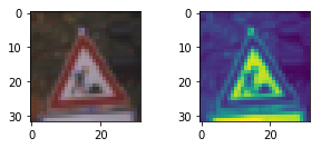
As a first step, I decided to convert the images to grayscale with opencv's function cv2.cvtColor(img, cv2.COLOR_BGR2GRAY) in order to remove flatten the shape of the image to 32x32x1
Here is an example of a traffic sign image before and after grayscaling.
As a last step, I normalized the image data with (pixel - 128.0) / 128.0 because then the mean is as close to 0 as possible.
Final Model Architecture
I started out with the original LeNet convnet as taught during the class but the best validation set accuracy I could achieve was around 93.3%. I started reading the paper – recommended by Udacity – published by Pierre Sermanet and Yann LeCun about a 2-stage convnet architecture specifically to recognize traffic signs. So after implementing it, the modified LeNet convnet architecture looks as follows:
| Layer | Description |
|---|---|
| Input | 32x32x1 grayscale image |
| Convolution 5x5 | 1x1 stride, valid padding, outputs 28x28x6 |
| RELU | |
| Max pooling | 2x2 stride, outputs 14x14x6 |
| Convolution 5x5 | 1x1 stride, valid padding, outputs 10x10x16 |
| RELU | |
| Max pooling | 2x2 stride, outputs 5x5x16 |
| Branch out | |
| 1. Branch | |
| Input | 5x5x16 |
| Convolution 5x5 | 1x1 stride, valid padding, outputs 1x1x400 |
| RELU | |
| Flatten | outputs 400 |
| 2. Branch | |
| Input | 5x5x16 |
| Flatten | outputs 400 |
| Concatenate | |
| Concatenate | inputs 2x400, outputs 800 |
| Dropout | keep prob of 50% |
| Fully connected | input 800, outpus 43 |
Training the model
To train the model, I used an Adam Optimizer to minimize the training loss. In addition, I set the parameters for the model as follows:
- Epochs: 30
- Batch size: 100
- Learning rate: 0.001
- Keep probability: 0.5
- Mean: 0
- Standard Deviation: 0.1
However, I tried a lot of variations of these parameters, see Progress in the Juypter Notebook.
Discussing the approach
My final model results were:
- validation set accuracy of 94.3%
- test set accuracy of 93.7%
I experimented quite a lot with two models – the classic LeNet5 and a modified LeNet described in the afforementioned research paper by Sermanet and LeCun.
-
2017/06/10 89.1%
- preprocessing: normalization
- model: LeNet, batch size: 128, epochs: 10, rate: 0.001, mu: 0, sigma: 0.1
-
2017/06/11 91.6%
- preprocessing: normalization grayscale
- model: LeNet, batch size: 150, epochs: 10, rate: 0.001, mu: 0, sigma: 0.1
-
2017/06/11 93.3%
- add dropout to LeNet
- preprocessing: normalization grayscale
- model: LeNet, batch size: 150, epochs: 10, rate: 0.001, mu: 0, sigma: 0.1, keep_prob: 0.5
-
2017/06/11 90.8%
- preprocessing: normalization grayscale
- modified LeNet according to research paper
- convolution 32x32x1 to 28x28x6
- subsampling (maxpooling) 28x28x6 to 14x14x6
- convolution 14x14x6 to 10x10x16
- subsampling (maxpooling) 10x10x16 to 5x5x16
- branch out
- branch:
- convolution 5x5x16 to 1x1x400
- flatten 1x1x400 to 400
- branch:
- flatten 5x5x16 to 400
- branch:
- concatenate 2 branches to 800
- fully connected
- model: ModLeNet, batch size: 128, epochs: 10, rate: 0.001, mu: 0, sigma: 0.1
-
2017/06/11 93.9%
- add dropout to ModLeNet
- preprocessing: normalization grayscale
- model: ModLeNet, batch size: 128, epochs: 10, rate: 0.001, mu: 0, sigma: 0.1, keep_prob: 0.5
-
2017/06/11 94.2%
- decreased learning rate and increased epochs
- preprocessing: normalization grayscale
- model: ModLeNet, batch size: 128, epochs: 20, rate: 0.0005, mu: 0, sigma: 0.1, keep_prob: 0.5
-
2017/06/11 95.2%
- increased learning rate, increased epochs, increased batch size
- preprocessing: normalization grayscale
- model: ModLeNet, batch size: 150, epochs: 30, rate: 0.0008, mu: 0, sigma: 0.1, keep_prob: 0.5
-
2017/06/11 95.3%
- decreased batch size
- preprocessing: normalization grayscale
- model: ModLeNet, batch size: 100, epochs: 30, rate: 0.0008, mu: 0, sigma: 0.1, keep_prob: 0.5
-
2017/06/11 94.3%
- increase learning rate
- preprocessing: normalization grayscale
- model: ModLeNet, batch size: 100, epochs: 30, rate: 0.001, mu: 0, sigma: 0.1, keep_prob: 0.5
I believe the modified LeNet works well for the problem of classifying traffic signs. It takes an unorthodox approach of branching out the data after stage 1 and passing part of the result straight to the output classifier. The dropout operation also increases the accuracy of the model tremendously. I could have probably increased the batch size and increased the epochs a little more and kept the learning rate between 0.001 and 0.0005. I have not experimented with different probabilities for keep_prob.
Qualities of new traffic sign images
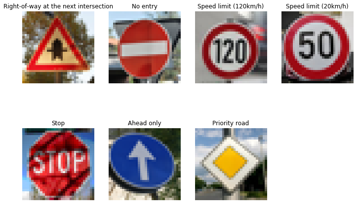
Here are seven German traffic signs that I found on the web:
I cropped and resized the images to fit the 32x32x3 dimensions the model requires as input. So all seven images are of good enough quality to be recognized by the trained classifier. However the "No Entry" sign has a sign of triangular shape behind it. So that might be tricky to classify correctly. Also the "Stop" sign has considerable shade making it hard to read even for a human being.
Model's predictions
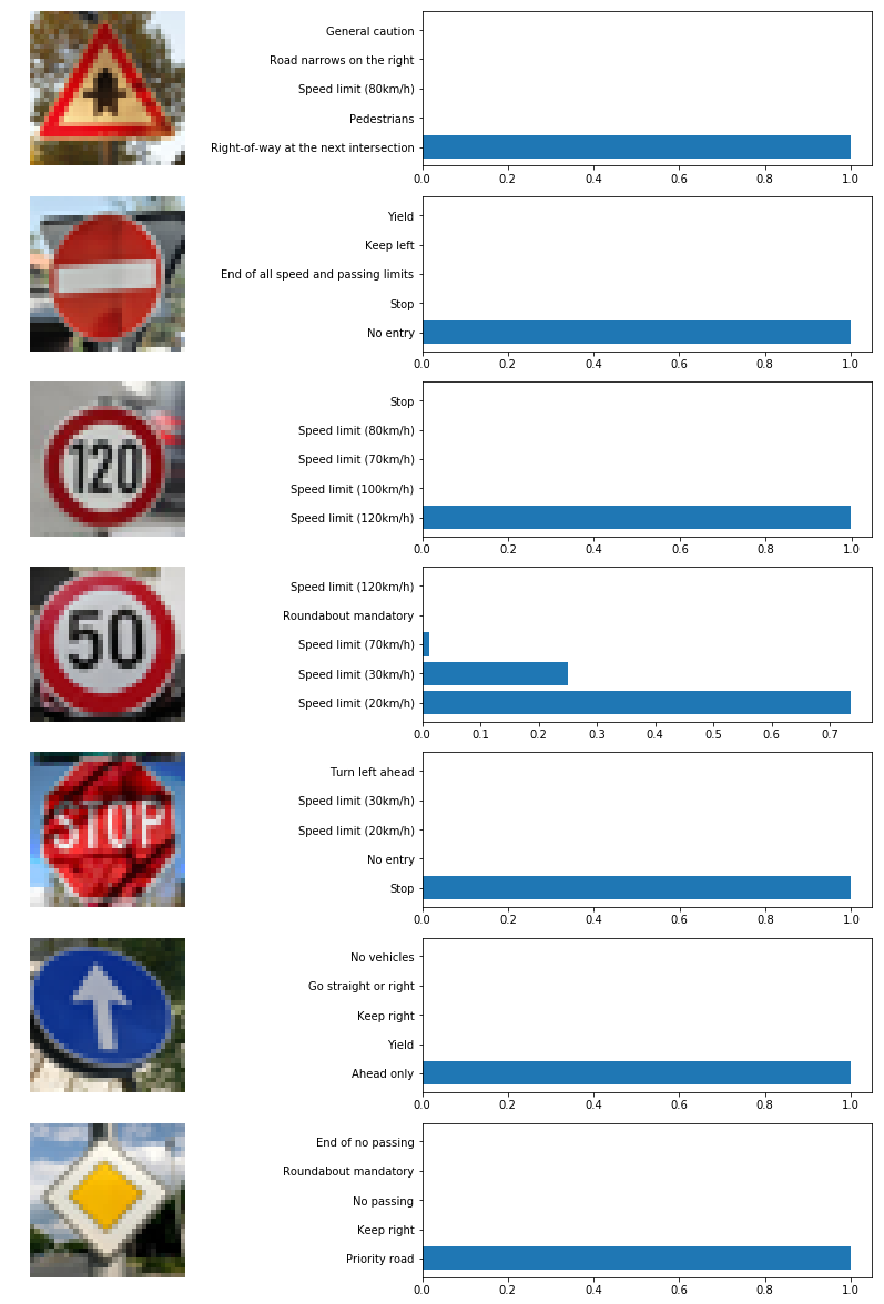
Here are the results of the prediction:
The accuracy of the predictions is a consolidated 85.7% compared to an accuracy of 93.7% on the test set. Of course the test set has 12000+ images and I'm testing on 7 images so it's actually not a bad result. Only 1 of the 7 images was misclassified.
Certainty of model's predictions
The model is 100% sure on all the images except the "Speed Limit (50km/h)" image. I find that very odd because it seems to be one of the clearest images of the seven. I can only explain that there's something wrong with the image and it is not noticable by the naked eye.
It's great that the classifier is not 100% correct, because that means there is still work to do on improving the convnet and classifier.


