Network Analytics Assignment
library(igraph)
library(tidyverse)
library(dplyr)
library(skimr)
library(ggplot2)
library(stringr)
library(scales)
library(psych)
Attaching package: ‘psych’


The following objects are masked from ‘package:scales’:

    alpha, rescale


The following objects are masked from ‘package:ggplot2’:

    %+%, alpha
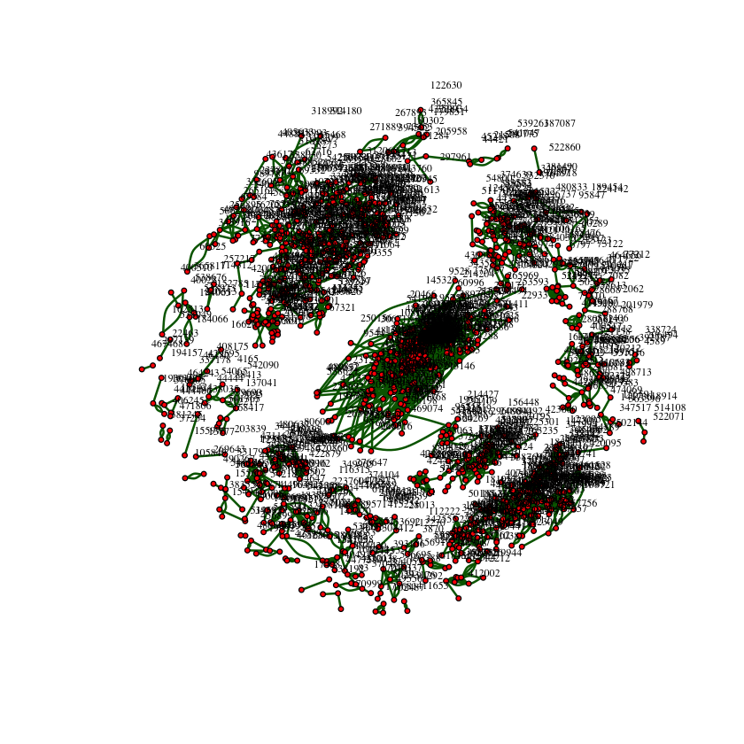
Plot the network using the information in the file graph subset rank1000.txt. Note that this is not the complete network, but only a subset of edges between top-ranked products. By visualizing the graph, you get an idea of the structure of the network you will be working on. In addition to plotting, comment on anything interesting you observe
graph1 <- read.graph(file="/Users/mhlaghari/Downloads/data 3/graph_subset_rank1000.txt", format ="ncol")#1355 nodes; 2611 edges
graph1IGRAPH 6421fc9 UN-- 1355 2611 --
+ attr: name (v/c)
+ edges from 6421fc9 (vertex names):
[1] 411653--94292 68951 --478494 236897--265343 236897--265343 236897--472765
[6] 153184--172503 172503--424919 469074--48638 48638 --480433 220748--42974
[11] 220748--42974 491768--105110 105110--291610 491768--105110 67371 --78848
[16] 120884--390297 390297--212405 355494--325446 29203 --349384 349384--20195
[21] 349384--444150 349384--285340 5039 --246337 325446--21728 21728 --530653
[26] 21728 --265598 355494--21728 216323--354795 45094 --96553 45094 --96553
[31] 342416--49527 445728--363808 267451--30639 287962--20466 153184--172503
[36] 153184--265468 153184--88060 153184--401507 153184--424919 153184--353676
+ ... omitted several edges
#to verify nodes and edges
cat("Nodes: ", vcount(graph1),"\n") #for nodes
cat("Edges: ", ecount(graph1)) #for edges
Nodes: 1355
Edges: 2611
#Get nodes
V(graph1)
+ 1355/1355 vertices, named, from 6421fc9:
[1] 411653 94292 68951 478494 236897 265343 472765 153184 172503 424919
[11] 469074 48638 480433 220748 42974 491768 105110 291610 67371 78848
[21] 120884 390297 212405 355494 325446 29203 349384 20195 444150 285340
[31] 5039 246337 21728 530653 265598 216323 354795 45094 96553 342416
[41] 49527 445728 363808 267451 30639 287962 20466 265468 88060 401507
[51] 353676 443284 33304 95210 124568 17994 374639 48316 535849 367733
[61] 83582 30695 468264 84492 225301 572 87559 315493 54800 488883
[71] 337679 209067 97692 35109 531651 108364 108187 13198 25341 65731
[81] 117196 62210 178132 144372 458306 324938 214842 197455 334110 61751
[91] 397309 97533 429060 100805 61718 313421 420909 514999 281633 178948
+ ... omitted several vertices
#Get Edges
E(graph1)
+ 2611/2611 edges from 6421fc9 (vertex names):
[1] 411653--94292 68951 --478494 236897--265343 236897--265343 236897--472765
[6] 153184--172503 172503--424919 469074--48638 48638 --480433 220748--42974
[11] 220748--42974 491768--105110 105110--291610 491768--105110 67371 --78848
[16] 120884--390297 390297--212405 355494--325446 29203 --349384 349384--20195
[21] 349384--444150 349384--285340 5039 --246337 325446--21728 21728 --530653
[26] 21728 --265598 355494--21728 216323--354795 45094 --96553 45094 --96553
[31] 342416--49527 445728--363808 267451--30639 287962--20466 153184--172503
[36] 153184--265468 153184--88060 153184--401507 153184--424919 153184--353676
[41] 153184--443284 153184--33304 153184--95210 124568--17994 17994 --374639
[46] 17994 --48316 17994 --535849 17994 --367733 124568--367733 83582 --30695
+ ... omitted several edges
#is the graph directed?
is.directed(graph1)
FALSE
plot.igraph(graph1,layout=layout.kamada.kawai,
            edge.width= 2,
            edge.color="darkgreen",
            vertex.color="red",
            vertex.size=2,
            vertex.label.color="black",
            vertex.label.cex=0.6,
            vertex.label.dist=2)
The graph isn't fully connected
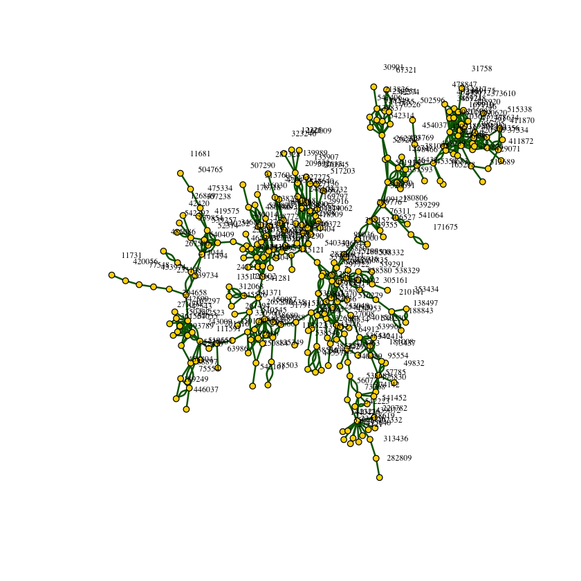
Now, use the file graph subset rank1000 cc.txt to plot only the largest connected component in the above network. You should be able to reuse your code from above on the new data.
graph2 <- read.graph(file="/Users/mhlaghari/Downloads/data 3/graph_subset_rank1000_cc.txt", format ="ncol")
graph2
IGRAPH b93f607 UN-- 292 604 --
+ attr: name (v/c)
+ edges from b93f607 (vertex names):
[1] 415305--112822 297722--116802 116802--182411 539734--273044 273044--267500
[6] 539367--538785 538785--538546 540230--540153 540153--539964 540153--516279
[11] 540230--540153 540230--542414 540230--539964 171675--541064 539367--538785
[16] 415305--539367 539367--447339 539367--82836 539367--48611 73768 --274142
[21] 95554 --73437 540153--542414 540230--542414 542414--73437 539964--542414
[26] 542414--95554 75527 --426430 312068--128602 128602--135171 128602--241213
[31] 381095--12274 12274 --541914 12274 --198466 12274 --423769 12274 --1299
[36] 12274 --136432 12274 --529269 12274 --262229 312068--135171 128602--135171
+ ... omitted several edges
# Is the graph directed?
is.directed(graph2)
FALSE
cat("Nodes: ", vcount(graph2),"\n") #for nodes
cat("Edges: ", ecount(graph2)) #for edges
Nodes: 292
Edges: 604
plot.igraph(graph2,layout=layout.kamada.kawai,
            edge.width= 2,
            edge.color="darkgreen",
            vertex.color="gold",
            vertex.size=3,
            vertex.label.color="black",
            vertex.label.cex=0.6,
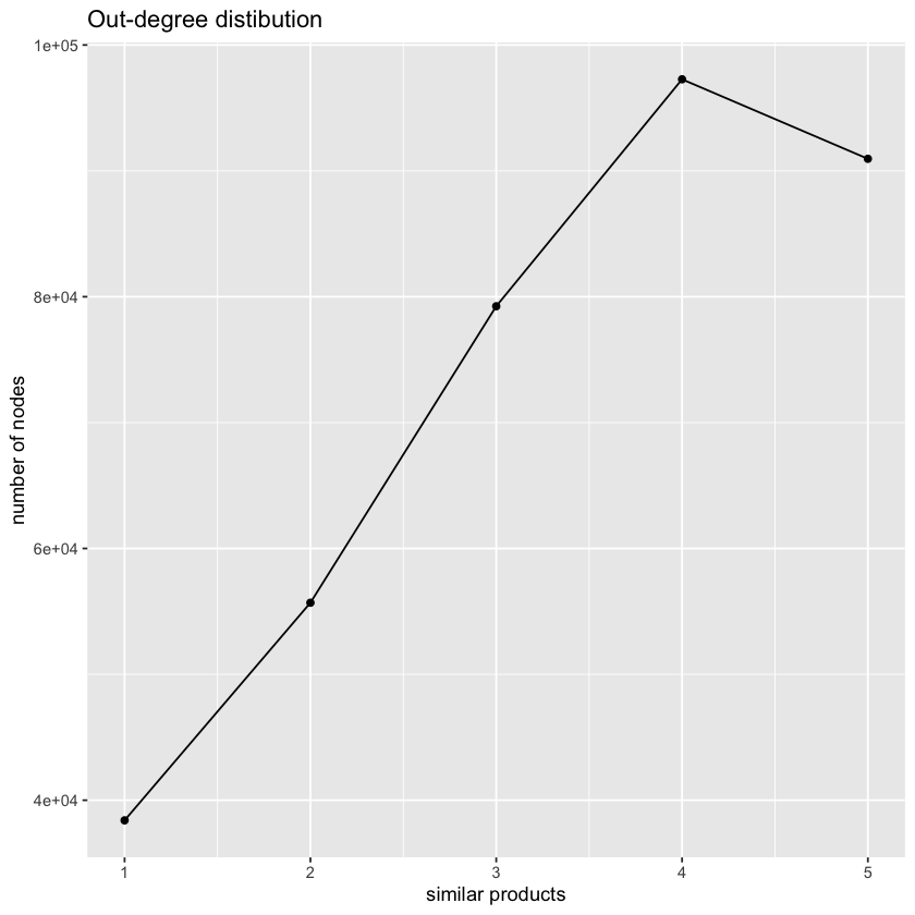
vertex.label.dist=2)Plot the out-degree distribution of our dataset (x-axis number of similar products, y-axis number of nodes). That is, for each product a, count the number of outgoing links to another product page b such that a → b.
Hint: The following steps will outline one way to approach this problem.
(a) Start by calculating the out-degree for each product. You may use the table command in R or a dict in Python to compute the number of outbound links for each product.
(b) You can then apply the same process you just used so that you can count the number of products (nodes) that have a particular number of outgoing links. This is the out-degree distribution.
(c) Once you are done, you can use the default plotting environment in R, ggplot2 in R,or matplotlib3 in Python to plot the distribution. Note that you can avoid step (b) if you use the geom density() function in ggplot or the hist() method in matplotlib.
However, you may approach this any way you wish.
data <- read.csv('/Users/mhlaghari/Downloads/data 3/graph_complete.txt', sep = ' ', header = FALSE)
id <- read.csv('/Users/mhlaghari/Downloads/data 3/id_to_titles.txt', sep=' ')
# create a directed graph
graph3 <- read.graph(file="/Users/mhlaghari/Downloads/data 3/graph_complete.txt", format ="ncol")
graph3 <- as.directed(graph3)
graph3IGRAPH fe81d46 DN-- 366987 2462800 --
+ attr: name (v/c)
+ edges from fe81d46 (vertex names):
[1] 140890->11405 11405 ->204319 1046 ->137479 137479->170475 183024->95075
[6] 95075 ->231749 405486->353453 272171->295744 295744->293925 295744->39760
[11] 295744->447055 295744->55313 295744->364778 295744->176964 295744->454565
[16] 295744->306149 295744->284831 272171->295744 272171->293925 272171->447055
[21] 272171->176964 272171->454565 272171->306149 39760 ->145536 55313 ->145536
[26] 284831->145536 295744->293925 272171->293925 293925->145536 293925->39760
[31] 293925->447055 293925->55313 293925->364778 293925->454565 293925->203692
[36] 293925->284831 293925->286635 293925->82947 39760 ->145536 39760 ->55313
+ ... omitted several edges
# Is the graph directed?
is.directed(graph3)
TRUE
cat("Nodes: ", vcount(graph3),"\n") #for nodes
cat("Edges: ", ecount(graph3)) #for edges
Nodes: 366987
Edges: 2462800
#method 1
#Step a
out1 <- table(data$V1)#Step b
out_degree <- data.frame(table(out1))
out_degree$out1<- as.numeric(out_degree$out1)#Step c
ggplot(out_degree ,aes(x=out1, y=Freq)) +
geom_point()+ geom_line()+
labs(x='similar products', y='number of nodes')+
ggtitle("Out-degree distibution")
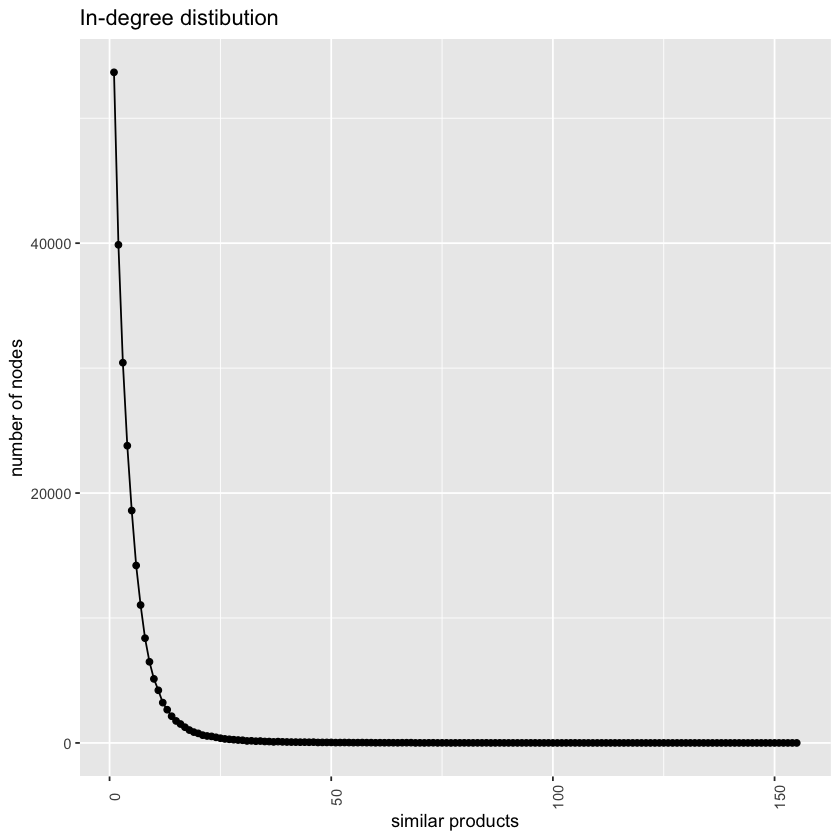
Above, you should have found that each product contains a maximum of five outbound links to similar products in the dataset. Now, plot the in-degree distribution of our dataset (x-axis number of similar products, y-axis number of nodes). That is, for each product a, count the number of incoming links from another product page b such that b → a. You can use the same steps outlined above. Is the distribution different? Comment on what you observe.
# step a
in1 <- table(data$V2)
# step b
in_degree <- data.frame(table(in1))
in_degree$in1<- as.numeric(in_degree$in1)# step c
ggplot(in_degree ,aes(x=in1, y=Freq), group=1) +
geom_point()+ geom_line()+
theme(axis.text.x = element_text(angle = 90))+
labs(x='similar products', y='number of nodes')+
ggtitle("In-degree distibution")OBSERVATION: The distribution is different most of the products have only one inbound link and the maximum number of inbound links is 549.
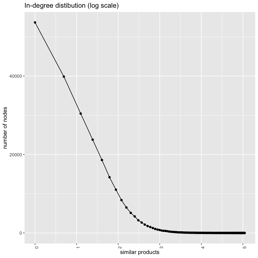
Transform the x-axis of the previous graph to log scale, to get a better understanding of the distribution. Note here that you should have some products with 0 inbound links. This means that using the log of the x-axis will fail since log(0) will not be valid. Due to this, you should replace 0 with 0.1. Comment on what you observe.
# plot previous graph by transforming x-axis to log scale

ggplot(in_degree ,aes(x=log(in1), y=Freq), group=1) +
  geom_point()+ geom_line()+
  theme(axis.text.x = element_text(angle = 90))+
  labs(x='similar products', y='number of nodes')+
ggtitle("In-degree distibution (log scale)")Compute the average number of inbound co-purchase links, the standard deviation, and the maximum. Comment on the result.
paste("The Average number of inbound co-purchase links is:",round(mean(in1), 1))
paste("The Standard deviation of inbound co-purchase links is:",round(sd(in1), 1))
paste("The maximum of inbound co-purchase links is:", max(in1))
'The Average number of inbound co-purchase links is: 5.2'
'The Standard deviation of inbound co-purchase links is: 6.8'
'The maximum of inbound co-purchase links is: 549'
Report the names of the 10 products with the most inbound co-purchase links
in1_df <- data.frame(in1)
in1_df$Var1<- as.numeric(in1_df$Var1)
# join in-degree data frame with Title
in_deg_title <- in1_df %>%inner_join(id, by = c("Var1" = "id"))# find top 10 product with the most inbound links
top10 <-as.data.frame(head(in_deg_title[order(in_deg_title$`Freq`, decreasing = T),],n=10))paste("The name of top 10 products with most inbound co-purchase are : ")
paste(top10$title, sep = '\n')'The name of top 10 products with most inbound co-purchase are : '
<style> .list-inline {list-style: none; margin:0; padding: 0} .list-inline>li {display: inline-block} .list-inline>li:not(:last-child)::after {content: "\00b7"; padding: 0 .5ex} </style>- 'Sacred Hoops : Spiritual Lessons of a Hardwood Warrior'
- 'Spiritual Warfare in a Believer\'s Life'
- 'Her Choice to Heal: Finding Spiritual and Emotional Peace After Abortion'
- 'No More Wacos: What\'s Wrong With Federal Law Enforcement and How to Fix It'
- 'Tables and Chairs (The Best of Fine Woodworking)'
- 'Killer Instincts: Anaconda - Giant Snake of the Amazon'
- 'The Inspector and Mrs. Jeffries (Victorian Mystery)'
- '0898'
- 'Improve Your Self Image (Love Tape/Audio Cassette)'
- 'Ortho\'s All About Landscaping Decks, Patios, and Balconies (Ortho\'s All About Gardening)'
