The concept of entropy is widely used in various machine learning methods. In this project we wanted to see, if this value behaves in the same way as an analogous quantity used in quantum physics - the entanglement entropy. To investigate this, we used both classical deep Q-learning and its quantum counterpart to train an agent to move in a simple Frozen Lake environment.
The output of a quantum circuit is of course a quantum state, for which the concept of entanglement entropy is pretty straightforward. In contrast, it's not as obvious in the case of classical RL. In that case, we were treating the output generated by the neural network as a quantum state (which in fact, is just some vector).
Q-learning is a machine learning algorithm of the "Reinforcement Learning" type. The family of such algorithms differs from supervised and unsupervised learning in that the information for training is collected not from data, but from the interaction of the agent (trained algorithm) with the environment. The function that the agent is guided by is called politics and takes the observation as an input (e.g. the position of a player on the board, car speed on the track) and returns an action (e.g. move right, add gas).
Further reading: https://en.wikipedia.org/wiki/Reinforcement_learning
We will explain the concept of Q-learning on the example of an agent moving around the "FrozenLake" environment. Let's take a 4x4 element board:
import gym

lake = gym.make('FrozenLake-v1', is_slippery=False)
lake.reset()
lake.render()
SFFF
FHFH
FFFH
HFFG
Legend:
- S: starting point, one per board,
- F: frozen surface - safe field,
- H: hole - an ice hole, a field that gives a large penalty, or ends the game,
- G: goal, end point.
The agent is always in one of the spaces and, based on his policy, decides to move in one direction (left, right, up, down). The entire walk focuses on the reward, which the agent increases or decreases by entering a specific field. Scoring example:
- Frozen surface: -0.01 to the reward (penalty to eliminate detour or walking in circles),
- Starting point: -0.01 to reward,
- Hole: -1 to the reward,
- End point: +1 to the reward.
Politics is a Q function that takes an action (e.g. move left) and a state (field 5 - second row from the top, second column from the right) as an input, and returns an appropriate reward. In the the most basic case (without the use of deep learning), the update of the politics (after each step) is represented by the Bellman equation:
Further reading: https://en.wikipedia.org/wiki/Q-learning
However, in our case, we use the so-called Deep Q-Learning (DQL). To make decisions, we use a neural network with a 16-element input (number of fields on the board) and a 4-element output, corresponding to the weights provided for each movement:
- 0 - move left,
- 1 - move down,
- 2 - move right,
- 3 - move up.
For example, if we would like to check which way is the best to go from the field number 5, we activate the neuron with index 4
We can access the exact values returned by the neural network as follows
agent.Qstate(4)tensor([0.4165, 0.6063, 0.5308, 0.4209])
We can see, that the second element is the greatest in value, so the agent is going to move downwards.
The whole thing was coded in pytorch. The architecture of our model is a network consisting of linear layers, followed by a sigmoid activation function:
- https://pytorch.org/docs/stable/generated/torch.nn.Sigmoid.html
- https://pytorch.org/docs/stable/generated/torch.nn.Linear.html
The loss function used was the SmoothL1Loss: https://pytorch.org/docs/stable/generated/torch.nn.SmoothL1Loss.html
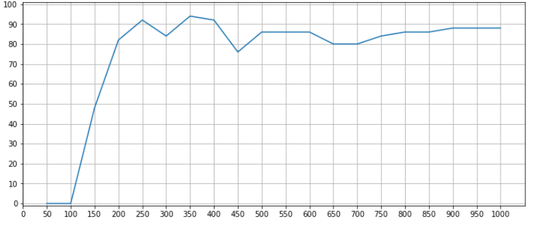
Several hundred epochs are enough to train a model. During the training we are tracking the percentage of cases, in which the walk ended up succesfully. For example, if the ratio of walks (over the last 50 epochs) during which the agent ended up in the goal field is equivalent to 90%, we are finishing the training process.
Below we present the average success rate over the last 50 epochs of training, during the total of 1000 epochs:
plt.figure(figsize=(12,5))
plt.plot(bin_stat.statistic)
plt.title(label=f'Percentage of succesfully finised walks (over the last {epoch_bin} epochs)')
plt.ylim(-1, 101)
plt.xlim(-1, (epochs+1)/epoch_bin)
plt.yticks(ticks=list(range(0, 110, 10)))
plt.xticks(ticks=bin_stat.bin_edges/epoch_bin-1, labels=bin_stat.bin_edges.astype(int))
plt.grid()
plt.show()
Additionally, we check whether the process is optimal or not. We strive for an algorithm that covers the route in 6 steps. If there is more of them, the algorithm is walking in circles. We are looking for the moment where it starts to oscillate around the optimal value. Therefore, we track how many steps an agent takes thanks to its politics, after each epoch:
plt.figure(figsize=(12,5))
plt.plot(t.jList)
plt.yticks(ticks=list(range(0, 110, 10)))
plt.title(label="Number of states done by the agent")
plt.grid()
plt.show()
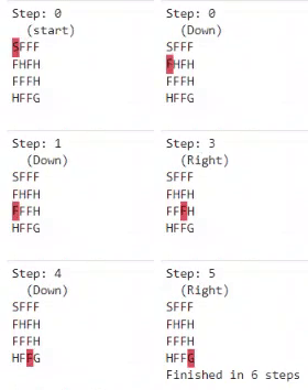
Let's see how the trained agent works:
In the quantum approach we are replacing the neural network with the so-called Variational Quantum Circuit (VQC). This is a type of quantum circuit with manipulable (classical) parameters. Like neural networks, VQCs can approximate arbitrary functions or classifiers. The following implementation is taken from
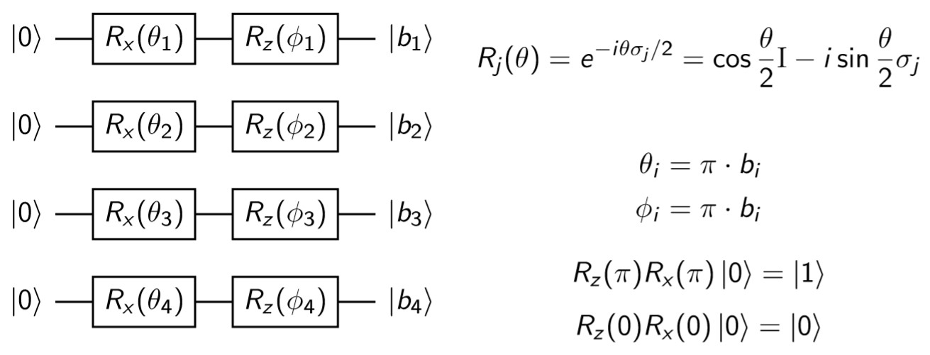
Recall that our task is, given a state (the place on the board where our agent is), to find the best corresponding move. The board contains 16 possible states (0-15), which can be encoded using 4 bits (0000-1111)
or similarly 4 qubits
For example, if we are in the 13th state, its bitwise representation is 1101, which can be also written down using qubits' states as .
Finally, the explicit gates which must be applied on consecutive qubits to encode agent's state are shown below:
Note, that we are using the and
parameters. These parameters won't be trained in the further part of the procedure, and are only used to encode the state properly.
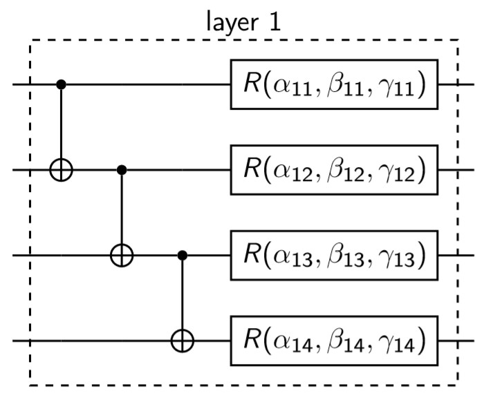
On the encoded state we are acting with the following gates:
At the beginning we are entangling all of the qubits using the CNOT gates. Then, we are rotating each qubit along the X, Y and Z axes according to the following formula
,
and
are the parameters that will be optimized during each training's iteration (which also means, that the gradient will be calculated exactly over these variables).
At the very end we are conducting a measurement of each qubit and basing on the output we make a proper move. The whole circuit looks as follows:
Because the training proces of VQC is very unstable we are (similarly as in the case of classical approach) using early stopping. We are terminating the procedure if during the last 20 epochs the reward didn't change and was positive.
It's important to note, that the state vector given by the VQC consists of complex variables, where n is the number of qubits, which in our case gives 16 numbers. To resemble this situation as close as possible we are extending the classical model by increasing the number of neurons in each layer (also the output one) to 32. We are using 32 real numbers to encode 16 complex ones.
It should be noted, that unfortunately due to this extension the agent's training becomes more unstable and converges more slowly.


