Jump to: Setup | Overview of the implementation | Running experiments | Results | Data sources
This repo contains an implementation of the Temporal Cluster Matching (TCM) algorithm and several baselines from the paper "Temporal Cluster Matching for Change Detection of Structures from Satellite Imagery". The Temporal Cluster Matching algorithm attempts to determine when a structure was constructed given that structure's footprint at a known point in time, as well as a time series of remotely sensed imagery leading up to that point in time. In the accompanying paper we use this algorithm with a dataset of poultry barn footprints from the Delmarva Peninsula in the US and dataset of solar farms footprints over the Indian state of Karnataka.
For a quick overview of the functionality implemented in this repo, see notebooks/Basic library function demos.ipynb.
If you make use of this implementation in your own project or want to refer to it in a scientific publication, please consider referencing this GitHub repository and citing our paper:
@inproceedings{robinsonTemporal2021,
  author  = {Caleb Robinson and Anthony Ortiz and Juan M. Lavista Ferres and Brandon Anderson and Daniel E. Ho},
  title   = {Temporal Cluster Matching for Change Detection of Structures from Satellite Imagery},
  year    = {2021},
  booktitle={Proceedings of the 4th ACM SIGCAS Conference on Computing and Sustainable Societies},
}
- 7/30/2021
-
Added a dataloader for Sentinel 2 imagery based on the Planetary Computer.
-
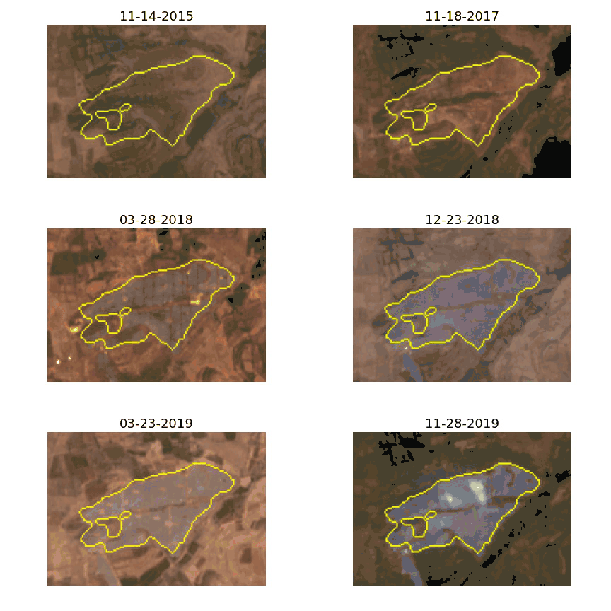
Added a notebook for demonstrating the new dataloader. This notebook downloads the time series of non-cloudy Sentinel 2 scenes for an input geometry and allows, for example, more precise change dates to be calculated.

-
Fixed a bug in
algorithms.calculate_change_values(if there were empty clusters then KL divergence value could be 'inf').
-
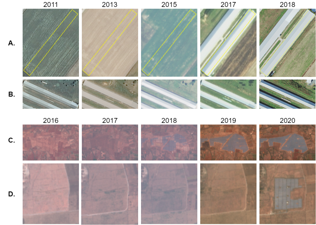
(A and B) Examples of two poultry barn footprints over 5 years of NAIP imagery. We observe inter-year variability of NAIP imagery and the change in the relation of color/texture between the footprint and neighborhood when a footprint is "developed". (C and D) Examples of two solar farm footprints over 5 years of Sentinel 2 imagery. Note, in A we outline the building footprint location in yellow through the entire series of imagery, but omit this outline in remaining rows.
First, run the following commands to create a conda environment, tcm, with the necessary dependencies for running the scripts and notebooks in this repository.
conda env create -f environment.yml
conda activate tcm
Then, download the Delmarva_PL_House_Final.zip file from the Soroka and Duren 2020 Poultry barn dataset from here. From the unzipped directory run:
conda activate tcm
ogr2ogr -of GeoJSON -t_srs epsg:4326 Delmarva_PL_House_Final2_epsg4326.geojson Delmarva_PL_House_Final2.shp
ogr2ogr -of GeoJSON -t_srs epsg:26918 Delmarva_PL_House_Final2_epsg26918.geojson Delmarva_PL_House_Final2.shp
Finally, copy the two generated files, Delmarva_PL_House_Final2_epsg4326.geojson and Delmarva_PL_House_Final2_epsg26918.geojson, to the data/ directory in this repository.
Our implementation of TCM is broken up into a data loader implementation and the main algorithm implementation.
For each dataset that we would like to run our algorithm on, we must implement a data loader class following the interface defined in the AbstractDataLoader. This class is repsonsible for interfacing with the remotely sensed imagery (i.e. grabbing patches of imagery over time around arbitrary footprints).
For example, we have implemented a NAIPDataLoader that can load a series of patches of NAIP imagery over time given an input geometry.
With this, the main algorithm implementation can be agnostic of the dataset we want to use.
The main algorithm implementation, i.e. the temporal_cluster_matching.algorithms.calculate_change_values(...) method, will return a list of KL-divergence values for a single footprint / series of imagery patches, then it is up to the user to use these in a decision function. In the paper we describe the main TCM algorithm with a decision threshold value (theta), as well as baselines that use the KL-divergence values in a logistic regression model. For an example of how these two parts of the implementation fit together, see [notebooks/Basic library function demos.ipynb](notebooks/Basic library function demos.ipynb).
The run_algorithm.py script is used to run the main algorithm implementation over a set of footprints with a given dataloader. For examples of this see the next section on running experiments.
To reproduce the main experiments we have included in the paper, first generate the KL-divergence values over the footprints for each dataset (as well over random polygons sampled from the respective AOIs):
python experiments/run_parameter_sweep_color.py # note, this will take a long time
python experiments/run_parameter_sweep.py # note, this will take even longer
As these take a long time to run, we have included the results of these runs in the repository already (see results/). You can reproduce a single run as:
python run_algorithm.py --dataset poultry_barns --num_clusters 32 --buffer 400 --output_dir results/kl/poultry_barns-32-400/ --algorithm kl
The second step is to generate predictions on when each footprint was constructed. See the following notebooks for examples that do this:
notebooks/Experiments - Learned theta and LR methods.ipynbnotebooks/Experiments - Heuristic method.ipynb
As mentioned in the previous section, we have included the results that we generated for the paper. The following is a list of the files containing these results and a brief description of how they were generated / what they contain:
results/poultry_barn_inter_year_color_distances.npy- Generated by
notebooks/Experiment - Color over time.ipynb. - This contains the differences in average footprint color between consecutive dates for each footprint in the poultry barn dataset.
- Generated by
results/solar_farm_inter_year_color_distances.npy- Generated by
notebooks/Experiment - Color over time.ipynb. - This contains the differences in average footprint color between consecutive dates for each footprint in the solar farm dataset.
- Generated by
results/heuristic-theta_results.csv- Generated by
notebooks/Experiments - Heuristic method.ipynb - This contains the Bhattacharyya coefficient, accuracy, and MAE results for each combination of {dataset, buffer, number of clusters} that we experiment with.
- Generated by
results/learned-theta_lr_results.csv- Generated by
notebooks/Experiments - Learned theta and LR methods.ipynb - This contains the accuracy and MAE results for each combination of {dataset, buffer, number of clusters} that we experiment with.
- Generated by
results/kl/*- Generated by
experiments/run_parameter_sweep.py - These are the raw output (i.e. list of KL divergences) for each combination of {dataset, buffer, number of clusters} that we experiment with using the TCM algorithm.
- Generated by
results/color/*- Generated by
experiments/run_parameter_sweep_color.py - These are the raw output (i.e. list of Euclidean distances) for each combination of {dataset, buffer, number of clusters} that we experiment with using the "Average-color" baseline.
- Generated by
This project uses two datasets, Poultry barns and Solar farms:
- The Poultry barns dataset is a public dataset from the USGS. See the following citation:
- Soroka, A.M., and Duren, Z., 2020, Poultry feeding operations on the Delaware, Maryland, and Virginia Peninsula from 2016 to 2017: U.S. Geological Survey data release, https://doi.org/10.5066/P9MO25Z7.
- The Solar farms dataset is a collection of model detected solar farms (polygons) over the Indian state of Karnataka, included as
data/karnataka_predictions_polygons_validated_2020.geojson.
The data/delmarva_valid_naip_area.geojson and data/solar_farms_valid_s2_area.geojson files give the spatial extent of these datasets. The data/naip_tiles_that_intersect_with_delmarva.txt file contains a list of NAIP tiles (with respect to the Azure Open Dataset NAIP catalog) that intersect with the spatial extent of the Poultry barns. The temporal_cluster_matching/DataInterface.py file contains methods for interfacing with the NAIP and Sentinel 2 imagery we use in each dataset. Finally, our manual construction date labels for these two datasets can be found in data/poultry_barn_labels.csv and data/solar_farm_labels.csv.
The data/poultry_barn_6013_random_polygons_epsg26918.geojson and data/solar_farms_935_random_polygons_epsg4326.geojson files contain the random selection of polygons over the two datasets used in our proposed heuristic method. These were generated by notebooks/Data - Create random polygons.ipynb.
This project is licensed under the MIT License.
