This is a short explanation on transformers.
Transformers was introduced in Attention is all you need back in 2017 as an alternative to Recurrent Neural Networks (RNN’s).RNN's treat sequences sequentially to keep the order of the sentence in place. To satisfy that design, each RNN component (layer) needs the previous (hidden) output. As such, stacked LSTM computations were performed sequentially. This is where transformers differ. The fundamental building block of a transformer is self-attention. Transformers feed the entire input sequence at once.
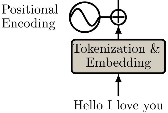
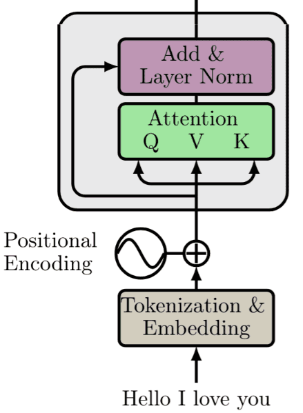
Before the input is fed to the model, 3 processing steps are performed.
In general, an embedding is a representation of a symbol (word, character, sentence) in a distributed low-dimensional space of continuous-valued vectors. Ideally, an embedding captures the semantics of the input by placing semantically similar inputs close together in the embedding space.

We will now provide some notion of order in the set through positional encodings.
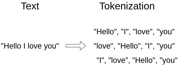
When you convert a sequence into a set (tokenization), you lose the notion of order. Since transformers process sequences as sets, they are, in theory, permutation invariant. Officially, positional encoding is a set of small constants, which are added to the word embedding vector before the first self-attention layer.
We try to provide some context to each word (token). o if the same word appears in a different position, the actual representation will be slightly different, depending on where it appears in the input sentence.
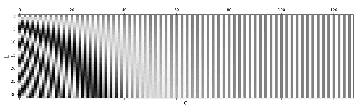
In the transformer paper, the authors came up with the sinusoidal function for the positional encoding. The sine function tells the model to pay attention to a particular wavelength . Given a signal
the wavelength will be
. In our case the λ will be dependent on the position in the sentence. i is used to distinguish between odd and even positions.
Mathematically:
This is in contrast to recurrent models, where we have an order but we are struggling to pay attention to tokens that are not close enough.
We now provide some necessary background information needed to understand some ideas introduced within the transformer architecture.
Key-value-query concepts come from information retrieval systems.This concept is important to grasp. Let's take youtube search as an example.
When you search (query) for a particular video, the search engine will map your query against a set of video titles, descriptions, etc. (keys) associated with stored videos. The algorithm then returns the best matched videos (values). This is the foundation of content/feature-based lookup.
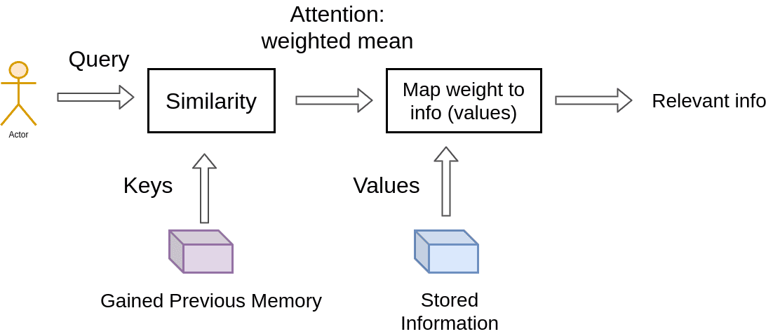
In the single video retrieval example, the attention is the choice of the video with a maximum relevance score. But we can relax this idea. To this end, the main difference between attention and retrieval systems is that we introduce a more abstract and smooth notion of ‘retrieving’ an object. By defining a degree of similarity (weight) between our representations (videos for youtube) we can weight our query. Instead of choosing where to look according to the position within a sequence, we now attend to the content that we wanna look at.
We use the keys to define the attention weights to look at the data and the values as the information that we will actually get. For the so-called mapping, we need to quantify similarity, that we will be seeing next.
In geometry, the inner vector product is interpreted as a vector projection. One way to define vector similarity is by computing the normalized inner product. In low dimensional space, like the 2D example below, this would correspond to the cosine value.
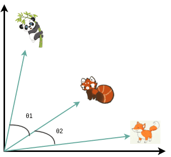
In transformers, this is the most basic operation and is handled by the self-attention layer as we’ll see.
''Self-attention, sometimes called intra-attention, is an attention mechanism relating different positions of a single sequence in order to compute a representation of the sequence.” ~ Ashish Vaswani et al. [2] from Google Brain''
Self-attention enables us to find correlations between different words of the input indicating the syntactic and contextual structure of the sentence.
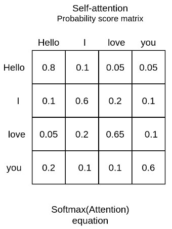
Let’s take the input sequence “Hello I love you” for example. A trained self-attention layer will associate the word “love” with the words ‘I” and “you” with a higher weight than the word “Hello”. From linguistics, we know that these words share a subject-verb-object relationship and that’s an intuitive way to understand what self-attention will capture.
In practice, the Transformer uses 3 different representations: the Queries, Keys and Values of the embedding matrix. This can easily be done by multiplying our input with 3 different weight matrices
. This is just a matrix multiplication in the original word embeddings. The resulted dimension will be smaller:
.
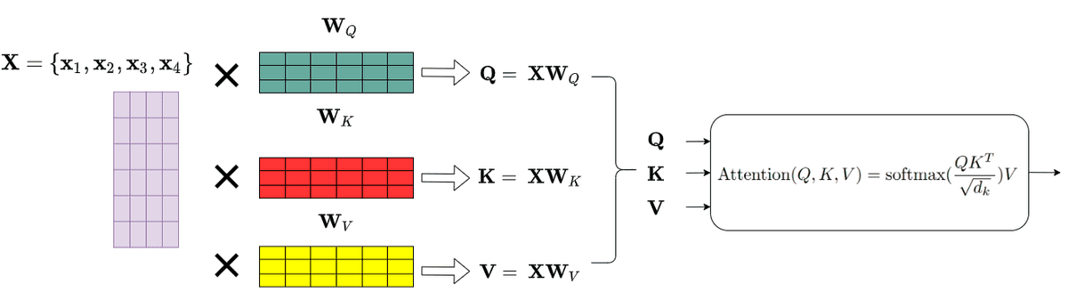
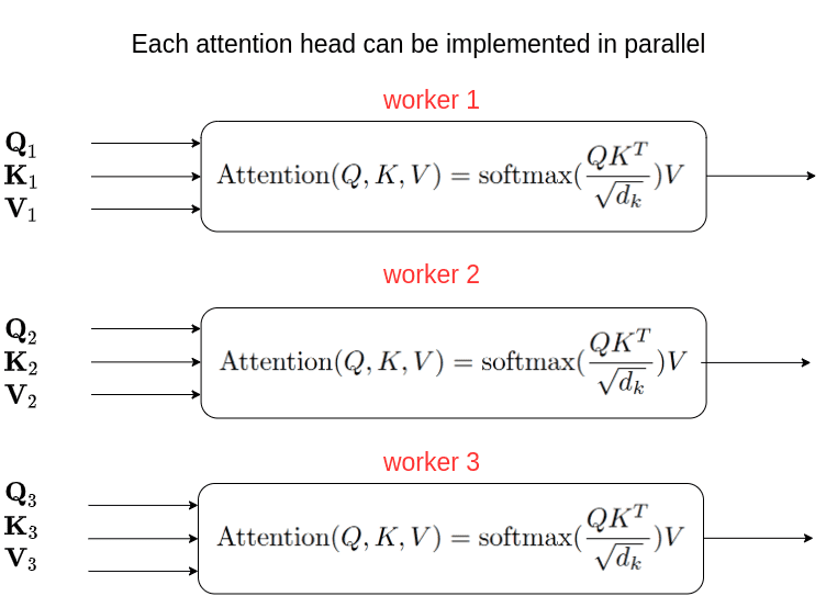
Having the Query, Value and Key matrices, we can now apply the self-attention layer as:
In the original paper, the scaled dot-product attention was chosen as a scoring function to represent the correlation between two words (the attention weight). Note that we can also utilize another similarity function. The is here simply as a scaling factor to make sure that the vectors won’t explode.
Following the database-query paradigm we introduced before, this term simply finds the similarity of the searching query with an entry in a database. Finally, we apply a softmax function to get the final attention weights as a probability distribution.
Remember that we have distinguished the Keys (K) from the Values (V) as distinct representations. Thus, the final representation is the self-attention matrix multiplied with the Value (V) matrix.
You can think of the attention matrix as where to look and the value matrix as what I actually want to get.
In the context of vector similarity, we have matrices instead of vectors and as a result matrix multiplications. We also don;t scale down by vector magnitude but by matrix size (d_k), which is the number of words in the sentence.
The next steps are normalization and skip connections, similar to processing a tensor after convolution or recurrency.
Skip connections give a transformer a tiny ability to allow the representations of different levels of processing to interact. With the forming of multiple paths, we can “pass” our higher-level understanding of the last layers to the previous layers. This allows us to re-modulate how we understand the input. For more information on skip connections.
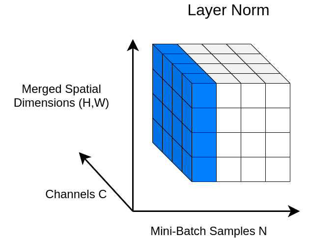
In Layer Normalization (LN), the mean and variance are computed across channels and spatial dims. In language, each word is a vector. Since we are dealing with vectors we only have one spatial dimension.
In a 4D tensor with merged spatial dimensions, we can visualize this with the following figure:
After applying a normalization layer and forming a residual skip connection we are here:
Even though this could be a stand-alone building block, the creators of the transformer add another linear layer on top and renormalize it along with another skip connection.
linear layer (PyTorch), dense layer (Keras), feed-forward layer (old ML books), fully connected layer. We will simply say linear layer which is:
Where W is a matrix and x,y,b are vectors. They add two linear layers with dropout and non-linearities in between.
import torch.nn as nn
dim = 512
dim_linear_block = 512*4

linear = nn.Sequential(
    nn.Linear(dim, dim_linear_block),
    nn.ReLU,
    nn.Dropout(dropout),
    nn.Linear(dim_linear_block, dim),
    nn.Dropout(dropout))
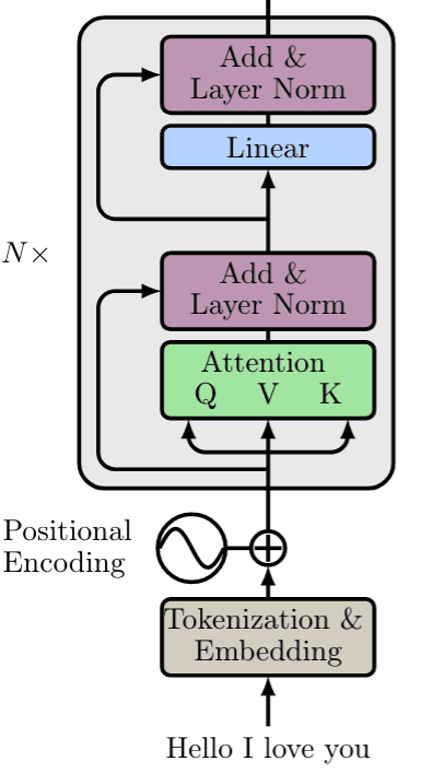
The main intuition is that they project the output of self-attention in a higher dimensional space (X4 in the paper). This solves bad initializations and rank collapse. We will depict it in the diagrams simply as Linear.
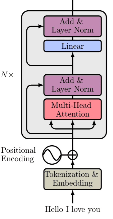
This (almost) concludes encoder part of the transformer with N such building blocks, as depicted below:
The final aspect to explore is multi-head attention
In the original paper, the authors expand on the idea of self-attention to multi-head attention. In essence, we run through the attention mechanism several times.
Each time, we map the independent set of Key, Query, Value matrices into different lower dimensional spaces and compute the attention there (the output is called a “head”). The mapping is achieved by multiplying each matrix with a separate weight matrix, denoted as .
To compensate for the extra complexity, the output vector size is divided by the number of heads. Specifically, in the vanilla transformer, they use model and h=8 heads, which gives us vector representations of 64. Now, the model has multiple independent paths (ways) to understand the input.
The heads are then concatenated and transformed using a square weight matrix since
Putting this together we get:
Since heads are independent from each other, we can perform the self-attention computation in parallel on different workers:
The intuition behind multihead attention is that it allows us to attend to different parts of the sequence differently each time. This practically means that:
- The model can better capture positional information because each head will attend to different segments of the input. The combination of them will give us a more robust representation.
- Each head will capture different contextual information as well, by correlating words in a unique manner.
''Multi-head attention allows the model to jointly attend to information from different representation subspaces at different positions. With a single attention head, averaging inhibits this.''
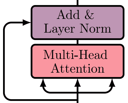
We will depict Multi-head self-attention in our diagrams like this:
Helpful resource on multihead attention: Pytorch implementation using the einsum notation.
Input is processed in 3 steps:
- Word embeddings of the input sentence are computed simultaneously.
- Positional encodings are then applied to each embedding resulting in word vectors that also include positional information.
- The word vectors are passed to the first encoder block.
Each block consists of the following layers in the same order:
-
A multi-head self-attention layer to find correlations between each word
-
A normalization layer
-
A residual connection around the previous two sublayers
-
A linear layer
-
A second normalization layer
-
A second residual connection
Note that the above block can be replicated several times to form the Encoder. In the original paper, the encoder composed of 6 identical blocks.
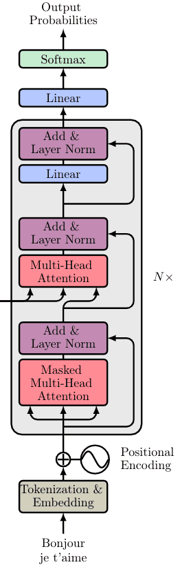
The decoder consists of all the aforementioned components plus two novel ones. As before:
-
The output sequence is fed in its entirety and word embeddings are computed
-
Positional encoding are again applied
-
And the vectors are passed to the first Decoder block
Each decoder block includes:
-
A Masked multi-head self-attention layer
-
A normalization layer followed by a residual connection
-
A new multi-head attention layer (known as Encoder-Decoder attention)
-
A second normalization layer and a residual connection
-
A linear layer and a third residual connection
The decoder block appears again 6 times. The final output is transformed through a final linear layer and the output probabilities are calculated with the standard softmax function.
The output probabilities predict the next token in the output sentence. How? In essence, we assign a probability to each word in the French language and we simply keep the one with the highest score.
To put things into perspective, the original model was trained on the WMT 2014 English-French dataset consisting of 36M sentences and 32000 tokens.
While most concepts of the decoder are already familiar, there are two more that we need to discuss. Let’s start with the Masked multi-head self-attention layer.
In case you haven’t realized, in the decoding stage, we predict one word (token) after another. In such NLP problems like machine translation, sequential token prediction is unavoidable. As a result, the self-attention layer needs to be modified in order to consider only the output sentence that has been generated so far.
In our translation example, the input of the decoder on the third pass will be “Bonjour”, “je” … …”.
As you can tell, the difference here is that we don’t know the whole sentence because it hasn’t been produced yet. That’s why we need to disregard the unknown words. Otherwise, the model would just copy the next word! To achieve this, we mask the next word embeddings (by setting them to −inf).
Mathematically we have:
where the matrix M (mask) consists of zeros and -inf. Zeros will become ones with the exponential while infinities become zeros.
This effectively has the same effect as removing the corresponding connection. The remaining principles are exactly the same as the encoder’s attention. And once again, we can implement them in parallel to speed up the computations.
Obviously, the mask will change for every new token we compute.
This is actually where the decoder processes the encoded representation. The attention matrix generated by the encoder is passed to another attention layer alongside the result of the previous Masked Multi-head attention block.
The intuition behind the encoder-decoder attention layer is to combine the input and output sentence. The encoder’s output encapsulates the final embedding of the input sentence. It is like our database. So we will use the encoder output to produce the Key and Value matrices. On the other hand, the output of the Masked Multi-head attention block contains the so far generated new sentence and is represented as the Query matrix in the attention layer. Again, it is the “search” in the database.
''The encoder-decoder attention is trained to associate the input sentence with the corresponding output word.'' It will eventually determine how related each English word is with respect to the French words. This is essentially where the mapping between English and French is happening.
Notice that the output of the last block of the encoder will be used in each decoder block.
- Distributed and independent representations at each block: Each transformer block has h=8 contextualized representations. Intuitively, you can think of it as the multiple feature maps of a convolution layer that capture different features from the image. The difference with convolutions is that here we have multiple views (linear reprojections) to other spaces. This is of course possible by initially representing words as vectors in a euclidean space (and not as discrete symbols).
- The meaning heavily depends on the context: This is exactly what self-attention is all about! We associate relationships between word representation expressed by the attention weights. There is no notion of locality since we naturally let the model make global associations.
- Multiple encoder and decoder blocks: With more layers, the model makes more abstract representations. Similar to stacking recurrent or convolution blocks we can stack multiple transformer blocks. The first block associates word-vector pairs, the second pairs of pairs, the third of pairs of pairs of pairs, and so on. In parallel, the multiple heads focus on different segments of the pairs. This is analogous to the receptive field but in terms of pairs of distributed representations.
- Combination of high and low-level information: Skip-connections enable top-down understanding to flow back with the multiple gradient paths that flow backward.
What is the difference between attention and a feedforward layer? Don't linear layers do exactly the same operations to an input vector as attention? No, You see the values of the self-attention weights are computed on the fly. They are data-dependent dynamic weights because they change dynamically in response to the data (fast weights).
For example, each word in the translated sequence (Bonjour, je t’aime) will attend differently with respect to the input.
On the other hand, the weights of a feedforward (linear) layer change very slowly with stochastic gradient descent. In convolutions, we further constrict the (slow) weight to have a fixed size, namely the kernel size.
Query vector is compared to a set of Key vectors and see how similar/compatible they are. Each Key vector comes paired with a value vector. They greater the compatibility of a given key with a query, the greater influence the corresponding value will have on the output of the attention mechanism. All Query, Keys and Values matrices are learned during training.
For each head of multi-head attention, the following happens:
- Each word in the input sequence is assigned a embedding. From each embedding, a key , query and value vector is extracted through linear transformations.
- Compatibility between Keys and Query matrices are determined through dot-product-attention. A greater dot product implies greater compatibility. We achieve a alpha vector of length the same size as the input sequence. This is a set of unnormalized weights and are normalized through a softmax, but first rescaled by the dimensionality of the query and key vectors d_k. This is done since the performance seems to suffer for larger values of d_k. This is hypothesized to be due to the softmax's gradient vanishing for high magnitude input. Variance of fot product grows with d_k and softmax gradient eventually vanishes. Thus dividing by the standard deviation helps counteract this.
- Once the attention weights are normalized, we create a linear combination of the value vectors and is the output of the attention mechanism.
- Similar to how each word token is mapped to a fixed sized vector embedding. Position tokens are assigned for this reason
- One way of doing this is by learnable lookup table for position tokens, the authors however proposed a handcrafted fixed encoding scheme
where D = 512.
- Each dimension follows a sinusoidal curve. Increasing in frequency as the dimension index i increases. Even dimension follows a sine curve and off an cosine curve.
Positional encodings have the same dim as input embeddings and are summed before feeding to the encoder.
- Vaswani, A., Shazeer, N., Parmar, N., Uszkoreit, J., Jones, L., Gomez, A. N., ... & Polosukhin, I. (2017). Attention is all you need. In Advances in neural information processing systems (pp. 5998-6008).
- DeepMind’s deep learning videos 2020 with UCL, Lecture: Deep Learning for Natural Language Processing, Felix Hill
- How Transformers work in deep learning and NLP: an intuitive introduction