Overview | Setup | Data | Usage | Licenses
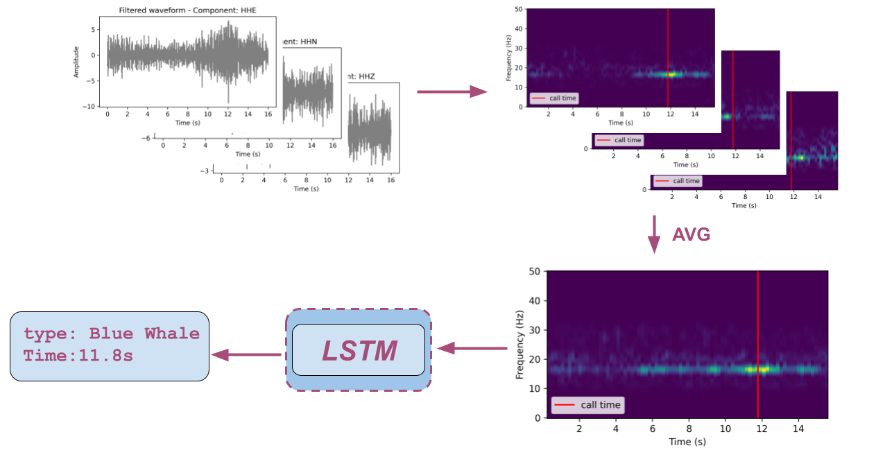
This repository implements a framework to detect whale calls embedded in seismic waveforms. Based on seismic waveform spectrogram, the algorithm performs the following two tasks:
- recognizing the presence of whale calls (classification task)
- predicting call time if recognized (regression task).

- Download and install the latest Anaconda Python distribution
- Download and uncompress the repository here.
- Execute the following commands to install all software requirements:
cd whale-call-detection
conda env create
pip install --editable .
- (Optional) Install pre-commits hooks:
cd whale-call-detection
conda activate whale
pre-commit install
- Download and install docker.
- Execute the following commands to install all software requirements to a Docker image:
cd whale-call-detection
docker build -t whale-call-detection .
The following commands will mount the current source code and provide access to the docker container's terminal:
cd whale-call-detection
docker run -it --rm \
    -v `pwd`:/home/whale-call-detection \
    -p 5000:5000 \
    -p 8888:8888 \
    whale-call-detection \
    /bin/bash
To use the GPU from within the Docker container, make sure to install nvidia-docker and set the Docker runtime to nvidia. For example:
cd whale-call-detection
docker run -it --rm --runtime=nvidia \
    -v `pwd`:/home/whale-call-detection \
    -p 5000:5000 \
    -p 8888:8888 \
    whale-call-detection \
    /bin/bash
The raw seismic data used in this study is publicly available via Natural Resoures Canada's FTP server: ftp://ftp.seismo.nrcan.gc.ca/. The labels (blue and fin whale calls) are generated using the algorithm and code developed by Plourde and Nedimovic [2022]. For more details on data availability and preprocesing, please check this documentation.
The directory format of processed waveform data is:
├── root_data_dir/
│   ├── 20200201/
│   │   ├── 2021.06.06.CN.CNQ..EHZ.SAC
        ├── 2021.06.06.CN.ICQ..HHE.SAC
        ├── ...
│   ├── 20200202/
│   │   ├── 2020.02.02.CN.CNQ..EHZ.SAC
        ├──2020.02.02.CN.ICQ..HHE.SAC
        ├── ...
│   ├── ...
│   │
The format of directory used to initialize an instance of WhaleDataModule is:
├── root_data_dir/
    ├── train.csv
    ├── valid.csv
    ├── test.csv
Here is the dataset dictionary:
| Column | Explanation | Type | Example |
|---|---|---|---|
file_path |
path to the .SAC file with its component replaced with CHANNEL
|
str |
/root_data_dir/20210822/2021.08.22.CN.SNFQ..CHANNEL.SAC |
time_window_start |
signal window start time | str |
2021-08-22 05:56:45.38 |
time_window_end |
signal window end time | str |
2021-08-22 05:57:01.38 |
time_R_max |
target call time, i.e. the time with the maximum whale index (R) value | str |
2021-08-22 05:56:54.01 |
time_call_start |
the start time of a whale call ( |
str |
2021-08-22 05:56:50.01 |
time_call_end |
the end time of a whale call ( |
str |
2021-08-22 05:56:58.01 |
R |
the whale call index value (fixed as 0.0 for noise samples) |
float |
19.7 |
SNR |
the signal-to-noise ratio of the whale call (fixed as -99.0 for noise samples |
float |
21.22 |
station_code |
station where the signal is detected | str |
SNFQ |
whale_type |
type of signal (0 for noise samples and 1 for a whale call |
int |
1 |
component |
list of components separated by space available for given station | str |
HHE HHN HHZ |
To split the dataset into train, validation and test datasets we have developped a script scripts/split_data.py.
python scripts/split_data.py -h
usage: split_data.py [-h] [--input-file INPUT_FILE] [--output-path OUTPUT_PATH]
Script to apply bandpass filter to a list of SAC files
optional arguments:
  -h, --help            show this help message and exit
  --input-file INPUT_FILE
                        Path to dataset (.csv) (default: data/LABELS/FW/MIXED/fw_HQ_component_grouped_filt.csv)
  --output-path OUTPUT_PATH
                        Path to output folder. (default: data/datasets/FWC_HQ_3CH_FILT/)
The dataset is split into 3 subsets using the same random seed: 80% for the training set, 10% for the validation set, and 10% for the test set.
To train a Long shot-term memory (LSTM) network, please check LSTM for more details. Samples of labels for training can be found here. Please note that raw waveform data is not included and can be downloaded following instructions in data.md.
To make prediction using a trained model (available here):
python scripts/predict.py -h
usage: predict.py [-h] [--model-ckpt MODEL_CKPT] [--inp-csv INP_CSV] [--out-csv OUT_CSV]
                  [--batch-size BATCH_SIZE]

Make prediction using a pretrained model

optional arguments:
  -h, --help            show this help message and exit
  --model-ckpt MODEL_CKPT
                        path to the pretrained model checkpoint (default: model.ckpt)
  --inp-csv INP_CSV     path to the input csv file (default: samples.csv)
  --out-csv OUT_CSV     path to the predictions csv file (default: predictions.csv)
  --batch-size BATCH_SIZE
                        batch size for prediction (default: 16)
The samples.csv has 4 columns: [file_path,time_window_start,time_window_end,component].
The predictions.csv has 6 columns: [ file_path,time_window_start,time_window_end,component,label_pred,time_pred].
Experiments are tracked using comet.
Please check this quickstart for more details on setup comet.
The hisory of experiments can be then visualized in your online Comet dashboard.
Optuna logs from a optuna.sqlite3 database located in the current directory can be consulted as follow:
optuna-dashboard sqlite:///optuna.sqlite3
Otherwise, Optuna logs can be consulted as follow:
optuna-dashboard sqlite:///ABSOLUTE_PATH_TO_OPTUNA.SQLITE3_FILE
Not applicable as no pre-trained modes are used.
- The seismograph data is licensed under the Open Government License - Canada.
| Package | Version | License |
|---|---|---|
| optuna | 3.1.0 | MIT License |
| optuna-dashboard | 0.10.0 | MIT License |
| pandas | 1.4.3 | BSD 3-Clause License |
| transformers | 4.20.1 | Apache 2.0 License |
| torchaudio | 0.12.1 | BSD 2-Clause License |
| torch | 1.12.1 | BSD 3-Clause License |
| pytorch_lightning | 1.9.2 | Apache2.0 |
| plotly | 5.9.0 | MIT License |
| obspy | 1.3.0 | LGPL v3.0 |
| matplotlib | 3.6.3 | Customized License |
| wget | 3.2 | GNU General Public License |
| types-pyyam | 6.0.12.6 | Apache 2.0 license |
| jsonargparse[signatures] | 4.20.0 | MIT License |
| wandb | 0.15.8 | MIT License |


