py-ciu

Explainable Machine Learning through Contextual Importance and Utility

NOTE: This python implementation is currently a work in progress. As such some of the functionality present in the original R version is not quite yet available.

The py-ciu library provides methods to generate post-hoc explanations for machine learning-based classifiers.

What is CIU?

Remark: It seems like Github Markdown doesn’t show correctly the “{” and “}” characters in Latex equations, whereas they are shown correctly in Rstudio. Therefore, in most cases where there is an $i$ shown in Github, it actually signifies {i} and where there is an $I$ it signifies {I}.

CIU is a model-agnostic method for producing outcome explanations of results of any “black-box” model y=f(x). CIU directly estimates two elements of explanation by observing the behaviour of the black-box model (without creating any “surrogate” model g of f(x)).

Contextual Importance (CI) answers the question: how much can the result (or the utility of it) change as a function of feature $i$ or a set of features ${i}$ jointly, in the context $x$?

Contextual Utility (CU) answers the question: how favorable is the value of feature $i$ (or a set of features ${i}$ jointly) for a good (high-utility) result, in the context $x$?

CI of one feature or a set of features (jointly) ${i}$ compared to a superset of features ${I}$ is defined as

$$ \omega_{j,{i},{I}}(x)=\frac{umax_{j}(x,{i})-umin_{j}(x,{i})}{umax_{j}(x,{I})-umin_{j}(x,{I})}, $$

where ${i} \subseteq {I}$ and ${I} \subseteq {1,\dots,n}$. $x$ is the instance/context to be explained and defines the values of input features that do not belong to ${i}$ or ${I}$. In practice, CI is calculated as:

$$ \omega_{j,{i},{I}}(x)= \frac{ymax_{j,{i}}(x)-ymin_{j,{i}}(x)}{ ymax_{j,{I}}(x)-ymin_{j,{I}}(x)}, $$

where $ymin_{j}()$ and $ymax_{j}()$ are the minimal and maximal $y_{j}$ values observed for output $j$.

CU is defined as

$$ CU_{j,{i}}(x)=\frac{u_{j}(x)-umin_{j,{i}}(x)}{umax_{j,{i}}(x)-umin_{j,{i}}(x)}. $$

When $u_{j}(y_{j})=Ay_{j}+b$, this can be written as:

$$ CU_{j,{i}}(x)=\left|\frac{ y_{j}(x)-yumin_{j,{i}}(x)}{ymax_{j,{i}}(x)-ymin_{j,{i}}(x)}\right|, $$

where $yumin=ymin$ if $A$ is positive and $yumin=ymax$ if $A$ is negative.

Usage

First, install the required dependencies. NOTE: this is to be run in your environment's terminal; some environments such as Google Colab might require an exclamation mark before the command, such as !pip install.

pip install py-ciu

Import the library:

from ciu import determine_ciu

Now, we can call the determine_ciu function which takes the following parameters:

case: A dictionary that contains the data of the case.
predictor: The prediction function of the black-box model py-ciu should call.
dataset: Dataset to deduct min_maxs from (dictionary). Defaults to None.
min_maxs (optional): dictionary ('feature_name': [min, max, is_int] for each feature), or infered from dataset. Defaults to None
samples (optional): The number of samples py-ciu will generate. Defaults to 1000.
prediction_index (optional): In case the model returns several predictions, it is possible to provide the index of the relevant prediction. Defaults to None.
category_mapping (optional): A mapping of one-hot encoded categorical variables to lists of categories and category names. Defaults to None.
feature_interactions (optional): A list of {key: list} tuples of features whose interactions should be evaluated. Defaults to [].

Here we can use a simple example with the well known Iris flower dataset

import pandas as pd
import numpy as np
from sklearn.model_selection import train_test_split
from sklearn import datasets
from sklearn.discriminant_analysis import LinearDiscriminantAnalysis

iris=datasets.load_iris()

df = pd.DataFrame(data = np.c_[iris['data'], iris['target']],
              columns = iris['feature_names'] + ['target'])
df['species'] = pd.Categorical.from_codes(iris.target, iris.target_names)
df.columns = ['s_length', 's_width', 'p_length', 'p_width', 'target', 'species']

X = df[['s_length', 's_width', 'p_length', 'p_width']]
y = df['species']
X_train, X_test, y_train, y_test = train_test_split(X, y, test_size=0.3, random_state=123)

Then create and train a model, in this case an LDA model

model = LinearDiscriminantAnalysis()
model.fit(X_train, y_train)

Now simply use our Iris flower data and the model, following the parameter descriptions above

iris_df = df.apply(pd.to_numeric, errors='ignore')

iris_ciu = determine_ciu(
    X_test.iloc[[42]],
    model.predict_proba,
    iris_df.to_dict('list'),
    samples = 1000,
    prediction_index = 2
)

Example Output

Let's import a test from the ciu_tests file

from ciu_tests.boston_gbm import get_boston_gbm_test

The get_boston_gbm_test function returns a CIU Object that we can simply store and use as such

boston_ciu = get_boston_gbm_test()
boston_ciu.explain_tabular()

Now we can also plot the CI/CU values using the CIU Object's plot_ciu function

boston_ciu.plot_ciu()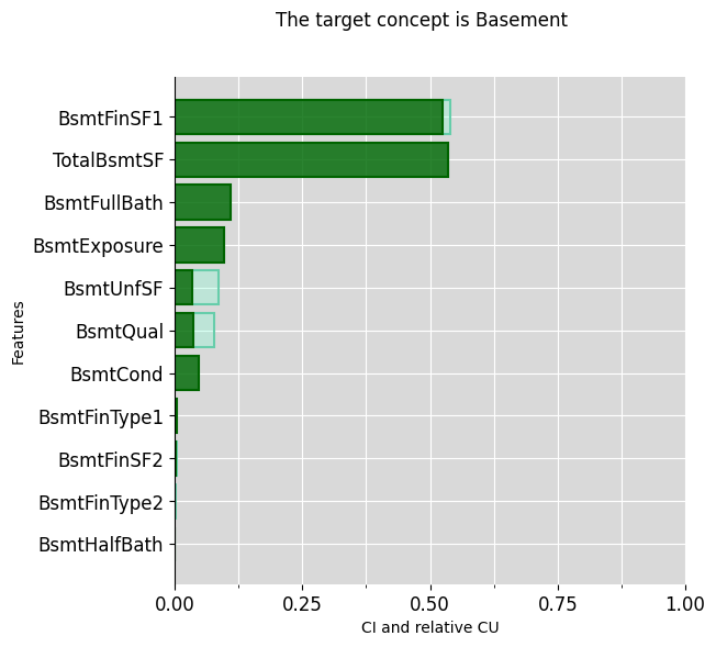

Likewise there are also several options available using the following parameters:

plot_mode: defines the type plot to use between 'default', 'overlap' and 'combined'.
include: defines whether to include interactions or not.
sort: defines the order of the plot bars by the 'ci' (default), 'cu' values or unsorted if None.
color_blind: defines accessible color maps to use for the plots, such as 'protanopia',
'deuteranopia' and 'tritanopia'.
color_edge_cu: defines the hex or named color for the CU edge in the overlap plot mode.
color_fill_cu: defines the hex or named color for the CU fill in the overlap plot mode.
color_edge_ci: defines the hex or named color for the CI edge in the overlap plot mode.
color_fill_ci: defines the hex or named color for the CI fill in the overlap plot mode.

Here's quick example using some of these parameters to create a modified version of the above plot

boston_ciu.plot_ciu(plot_mode="combined", color_blind='tritanopia', sort='cu')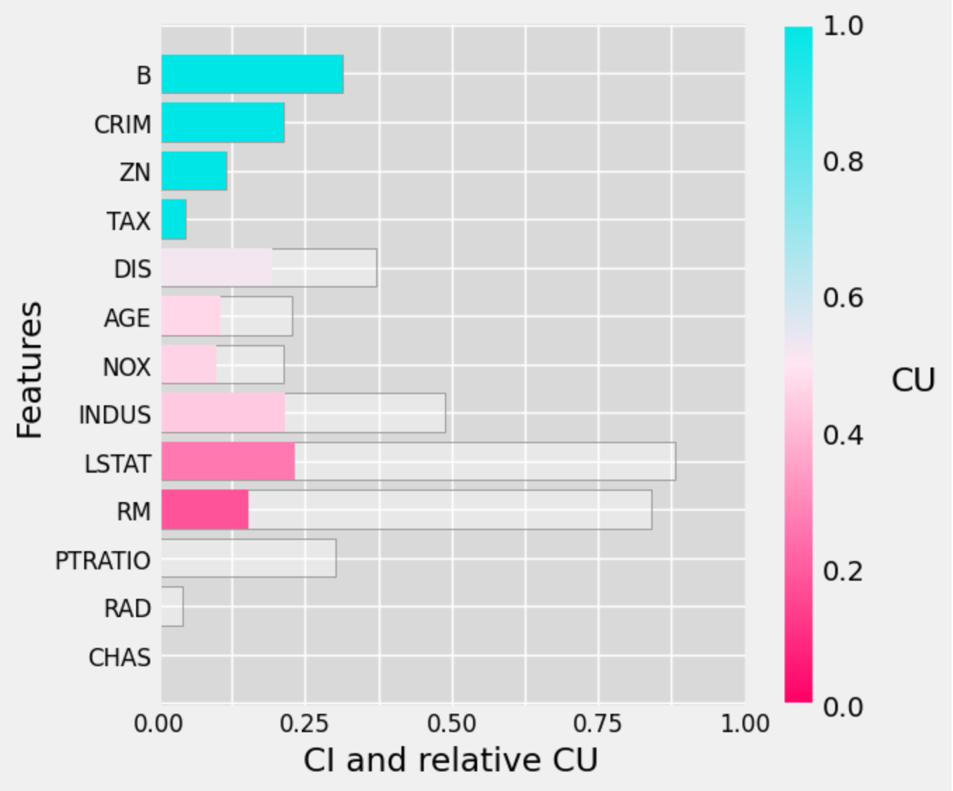

Contextual influence

Contextual influence and can be calculated from CI and CU as follows:

$$ \phi_{j,{i},{I}}(x)=\omega_{j,{i},{I}}(x)(CU_{j,{i}}(x) - \phi_{0}), $$

where $\phi_{0}$ is the baseline/reference value ($y(u(0))$ in the plot). For instance, $\phi_{0}=0.5$ signifies using the average utility value $0.5$ as the baseline, which is the case in the $age$ plot above. An explanation using Contextual influence on the titanic dataset can be obtained as follows:

Note: the dataset and model used are not identical to the R version, therefore the results will see a slight variance.

import pandas as pd
from sklearn.ensemble import RandomForestClassifier
from ciu.ciu_core import determine_ciu

data = pd.read_csv("https://raw.githubusercontent.com/KaryFramling/py-ciu/master/ciu_tests/data/titanic.csv")
data = data.drop(data.columns[0], axis=1)
unused = ['PassengerId','Cabin','Name','Ticket']

for col in unused:
    data = data.drop(col, axis=1)

from sklearn.preprocessing import LabelEncoder
data = data.dropna().apply(LabelEncoder().fit_transform)
train = data.drop('Survived', axis=1)

model = RandomForestClassifier(n_estimators=100)
model.fit(train, data.Survived)

Creating a new instance for the CIU Object

# Create test instance (8-year old boy)
new_passenger = pd.DataFrame.from_dict({"Pclass" : [1], "Sex": [1], "Age": [8], "SibSp": [0], "Parch": [0], "Fare": [72], "Embarked": [2]})

ciu_titanic = determine_ciu(
    new_passenger,
    model.predict_proba,
    train.to_dict('list'),
    samples = 1000,
    prediction_index = 1,
    intermediate_concepts=intermediate_tit
)

Output a barplot using Contextual Influence:

ciu_titanic.plot_ciu(use_influence=True, include_intermediate_concepts='no')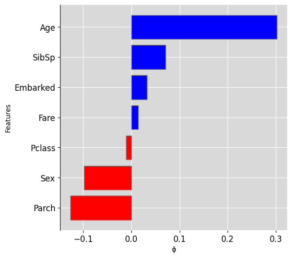

Remark: The Equation for Contextual influence is similar to the definition of Shapley values for linear models, except that the input value $x_{i}$ is replaced by its utility value(s) $CU_{j,{i}}(x)$. In practice, all Additive Feature Attribution (AFA) methods estimate influence values, not feature importance. Most state-of-the-art methods such as Shapley values, LIME, are AFA methods.

Influence values give no counter-factual information and are easily misinterpreted. Below, we create a Shapley value explanation using the IML package. In that explanation, for instance the close-to-zero Shapley value for $Parch$ gives the impression that it’s a non-important feature, which is clearly wrong based on the CIU explanation.

import shap
explainer = shap.Explainer(model, train)
shap_values = explainer(new_passenger)
shap.plots.bar(shap_values[0,:,1], order=np.argsort(shap_values[0,:,1].values)[::-1])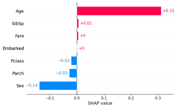

It might be worth mentioning also that the Shapley value explanation has a much greater variance than the CIU (and Contextual influence) explanation with same number of samples. This is presumably due to the fundamental difference between estimating min/max output values for CIU, compared to estimating a kind of gradient with AFA methods.

Intermediate Concepts

CIU can use named feature coalitions and structured vocabularies. Such vocabularies allow explanations at any abstraction level and can make explanations interactive.

The following code snippet plots the joint effect of features $age$ and $parch$ for the studied Titanic case (applicable for numeric features). It therefore shows how the coalition of those two features affects the output value and how CI and CU can be deduced in the same way as for a single feature.

ciu_titanic.plot_3D(ind_inputs=[4,2])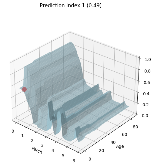

Titanic Example

We define a small vocabulary for Titanic as follows:

intermediate_tit = [
        {"Wealth":['Pclass', 'Fare']},
        {"Family":['SibSp', 'Parch']},
        {"Gender":['Sex']},
        {"Age_years":['Age']},
        {"Embarked_Place":['Embarked']}
    ]

Then we create a new CIU object that uses that vocabulary and get top-level explanation.

ciu_titanic = determine_ciu(
    new_passenger,
    model.predict_proba,
    train.to_dict('list'),
    samples = 1000,
    prediction_index = 1,
    intermediate_concepts=intermediate_tit
)

First barplot explanation:

ciu_titanic.plot_ciu(include_intermediate_concepts='only', plot_mode='overlap')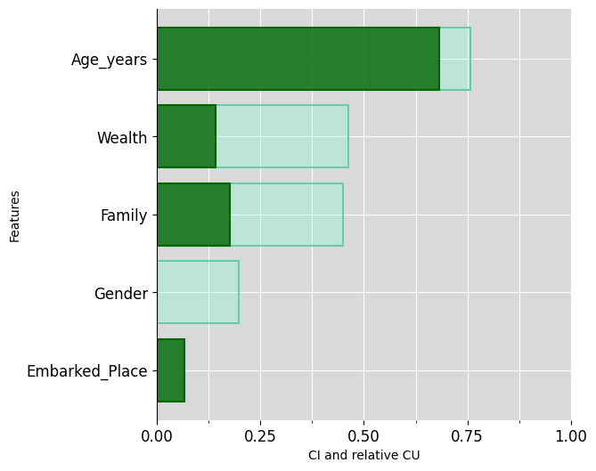

Then explain WEALTH and FAMILY

ciu_titanic.plot_ciu(target_concept="Family", plot_mode="overlap")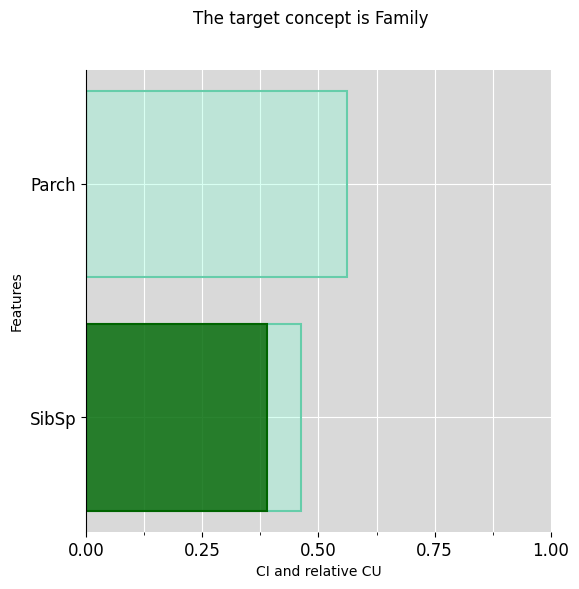

ciu_titanic.plot_ciu(target_concept="Wealth", plot_mode="overlap")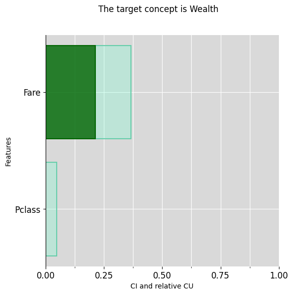

Same thing using textual explanations:

ciu_titanic.explain_text(include_intermediate_concepts="only")

## The feature "Wealth", which is of normal importance (CI=46.15%), is somewhat typical for its prediction (CU=30.95%).
## The feature "Family", which is of normal importance (CI=45.05%), is somewhat typical for its prediction (CU=39.02%).
## The feature "Gender", which is of very low importance (CI=19.76%), is not typical for its prediction (CU=0.1%).
## The feature "Age_years", which is of high importance (CI=75.82%), is very typical for its prediction (CU=89.86%).
## The feature "Embarked_Place", which is of very low importance (CI=6.59%), is very typical for its prediction (CU=100.0%)

ciu_titanic.explain_text(target_concept="Family")

## 'The intermediate concept "Family", is somewhat typical for its prediction (CU=39.02%).',
## 'The feature "SibSp", which is of normal importance (CI=46.34%), is very typical for its prediction (CU=84.21%).',
## 'The feature "Parch", which is of normal importance (CI=56.1%), is not typical for its prediction (CU=0.1%).'

ciu_titanic.explain_text(target_concept="Wealth")

## 'The intermediate concept "Wealth", is somewhat typical for its prediction (CU=30.95%).',
## 'The feature "Pclass", which is of very low importance (CI=4.76%), is not typical for its prediction (CU=0.1%).',
## 'The feature "Fare", which is of low importance (CI=36.51%), is typical for its prediction (CU=58.7%).'

Ames Housing Example

Ames housing is a data set about properties in the town Ames in the US. It contains over 80 features that can be used for learning to estimate the sales price. The following code imports the data set, does some pre-processing and trains a Gradient Boosting model:

from ciu.ciu_core import determine_ciu
import pandas as pd
import xgboost as xgb
from sklearn.model_selection import train_test_split

df = pd.read_csv('AmesHousing.csv')

#Checking for missing data
missing_data_count = df.isnull().sum()
missing_data_percent = df.isnull().sum() / len(df) * 100

missing_data = pd.DataFrame({
    'Count': missing_data_count,
    'Percent': missing_data_percent
})

missing_data = missing_data[missing_data.Count > 0]
missing_data.sort_values(by='Count', ascending=False, inplace=True)

#This one has spaces for some reason
df.columns = df.columns.str.replace(' ', '')


#Taking care of missing values
from sklearn.impute import SimpleImputer
# Group 1:
group_1 = [
    'PoolQC', 'MiscFeature', 'Alley', 'Fence', 'FireplaceQu', 'GarageType',
    'GarageFinish', 'GarageQual', 'GarageCond', 'BsmtQual', 'BsmtCond',
    'BsmtExposure', 'BsmtFinType1', 'BsmtFinType2', 'MasVnrType'
]
df[group_1] = df[group_1].fillna("None")

# Group 2:
group_2 = [
    'GarageArea', 'GarageCars', 'BsmtFinSF1', 'BsmtFinSF2', 'BsmtUnfSF',
    'TotalBsmtSF', 'BsmtFullBath', 'BsmtHalfBath', 'MasVnrArea'
]

df[group_2] = df[group_2].fillna(0)

# Group 3:
group_3a = [
    'Functional', 'MSZoning', 'Electrical', 'KitchenQual', 'Exterior1st',
    'Exterior2nd', 'SaleType', 'Utilities'
]

imputer = SimpleImputer(strategy='most_frequent')
df[group_3a] = pd.DataFrame(imputer.fit_transform(df[group_3a]), index=df.index)

df.LotFrontage = df.LotFrontage.fillna(df.LotFrontage.mean())
df.GarageYrBlt = df.GarageYrBlt.fillna(df.YearBuilt)

#Label encoding
from sklearn.preprocessing import LabelEncoder
df = df.apply(LabelEncoder().fit_transform)

data = df.drop(columns=['SalePrice'])
target = df.SalePrice

#Splitting and training
X_train, X_test, y_train, y_test = train_test_split(data, target, test_size=0.3, random_state=123)
xg_reg = xgb.XGBRegressor(objective ='reg:squarederror', colsample_bytree = 0.5, learning_rate = 0.1, max_depth = 15, alpha = 10)

xg_reg.fit(X_train,y_train)

Then we create our vocabulary of intermediate concepts, in this case a list containing dictionaries of a concept->[columns]structure as follows:

intermediate = [
    {"Garage":list(df.columns[[58,59,60,61,62,63]])},
    {"Basement":list(df.columns[[30,31,33,34,35,36,37,38,47,48]])},
    {"Lot":list(df.columns[[3,4,7,8,9,10,11]])},
    {"Access":list(df.columns[[13,14]])},
    {"House_type":list(df.columns[[1,15,16,21]])},
    {"House_aesthetics":list(df.columns[[22,23,24,25,26]])},
    {"House_condition":list(df.columns[[17,18,19,20,27,28]])},
    {"First_floor_surface":list(df.columns[[43]])},
    {"Above_ground_living area":[c for c in df.columns if 'GrLivArea' in c]}
]

Now we can initialise the CIU object with a relatively favourable test case and our newly defined intermediate concepts:

test_data_ames = X_test.iloc[[345]]

ciu = determine_ciu(
    test_data_ames,
    xg_reg.predict,
    df.to_dict('list'),
    samples = 1000,
    prediction_index = None,
    intermediate_concepts = intermediate
)

We start with an “explanation” using all 80 basic features, which is not very readable and overly detailed for “ordinary” humans to understand:

ciu_ames.plot_ciu(include_intermediate_concepts='no', plot_mode='overlap')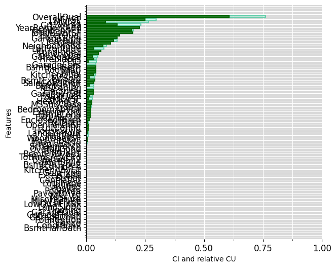

Then the same, using highest-level concepts:

ciu_ames.plot_ciu(include_intermediate_concepts='only', plot_mode='overlap')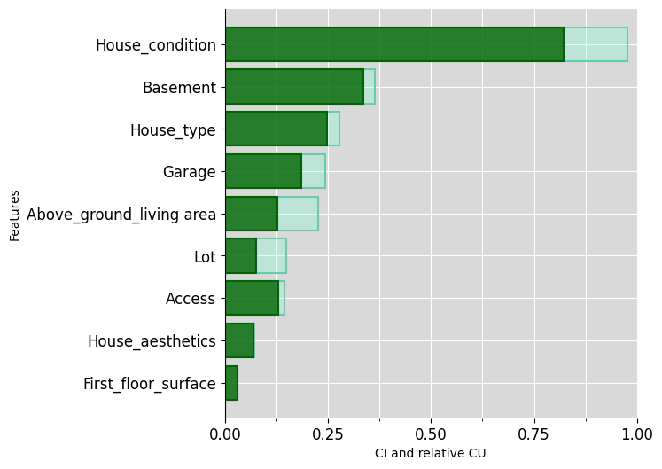

Then explain further some intermediate concepts:

ciu_ames.plot_ciu(target_concept="House_condition", plot_mode="overlap")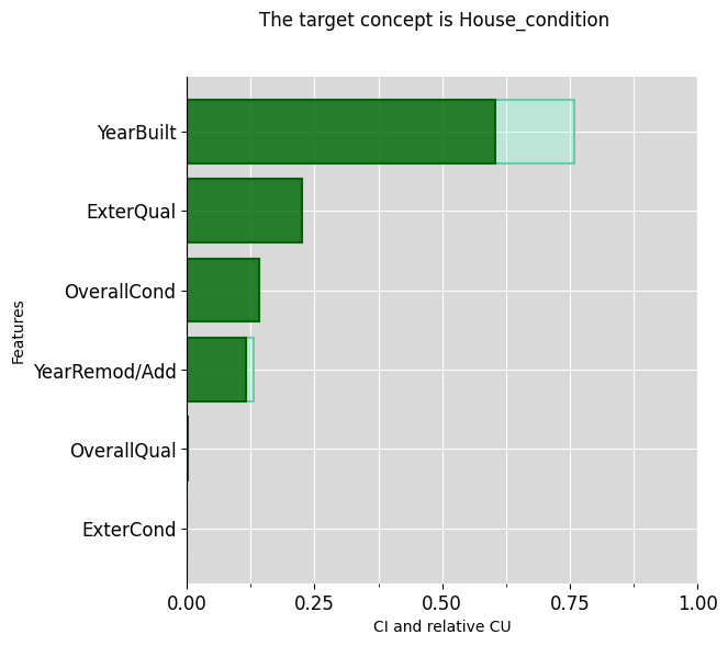

ciu_ames.plot_ciu(target_concept="Basement", plot_mode="overlap")

ciu_ames.plot_ciu(target_concept="Garage", plot_mode="overlap")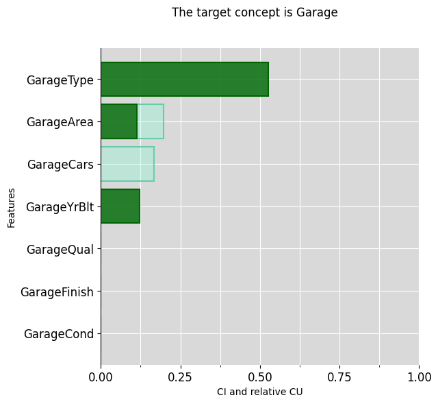

This vocabulary is just an example of what kind of concepts a human typically deals with. Vocabularies can be built freely (or learned, if possible) and used freely, even so that different vocabularies can be used with different users.

Related resources

The original R implementation can be found at: https://github.com/KaryFramling/ciu

There are also two implementations of CIU for explaining images:

Image explanation packages can be considered to be at proof-of-concept level (Nov. 2022). Future work on image explanation will presumably focus on the Python version, due to the extensive use of deep neural networks that tend to be implemented mainly for Python.

Authors

The current version of py-ciu re-uses research code provided by Timotheus Kampik and replaces it. The old code is available in the branch "Historical".

minalspatil/explainml