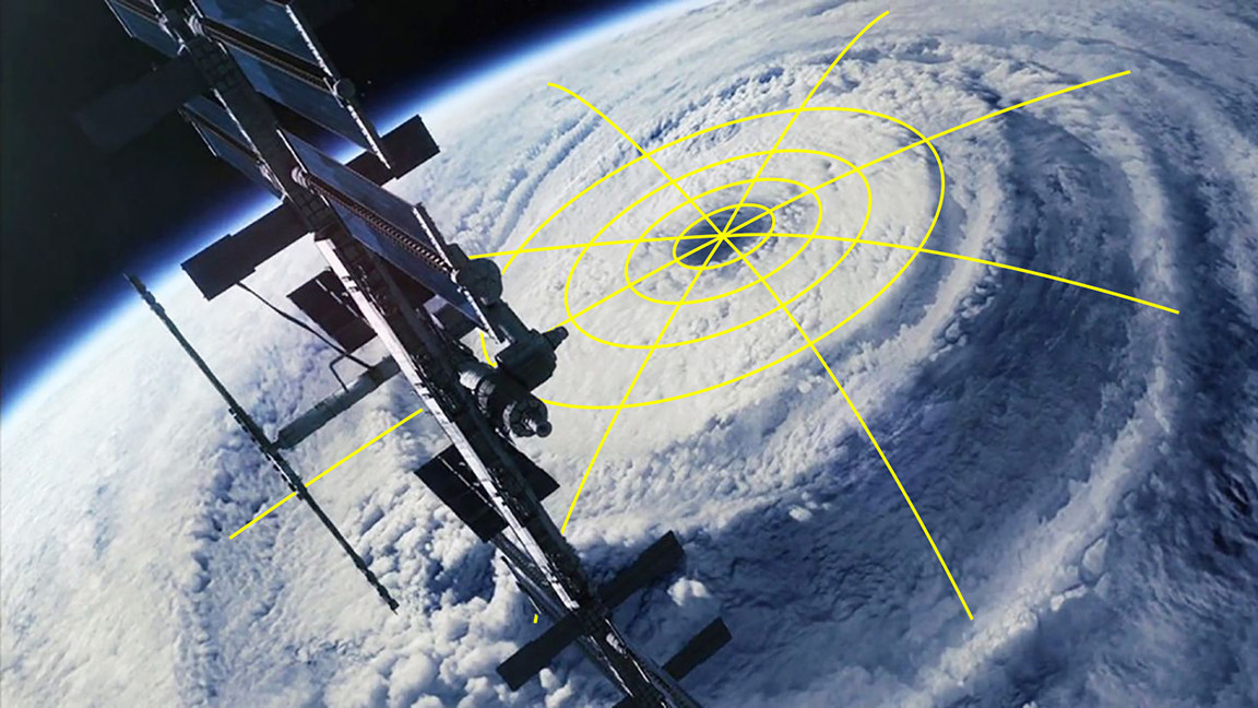
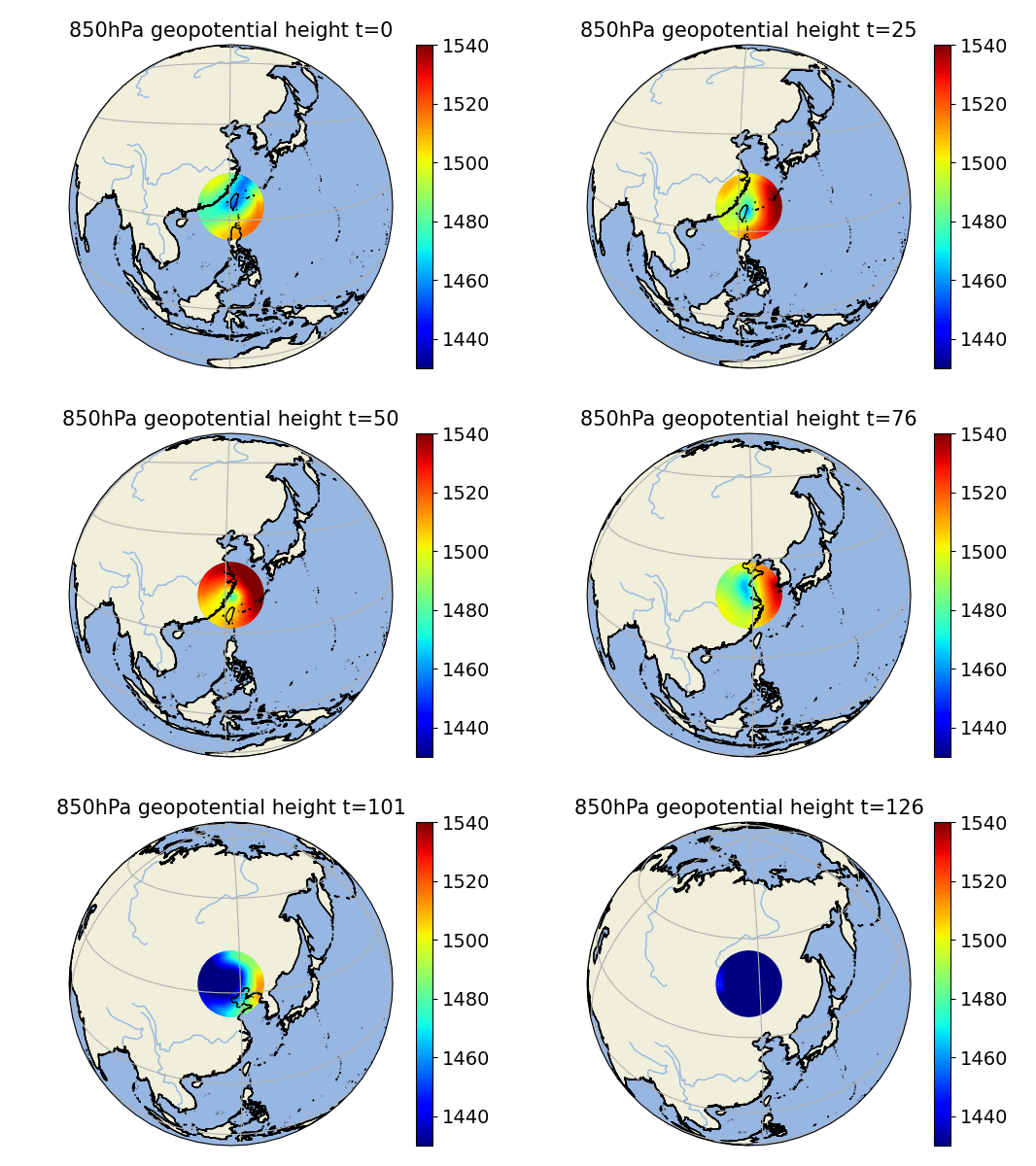
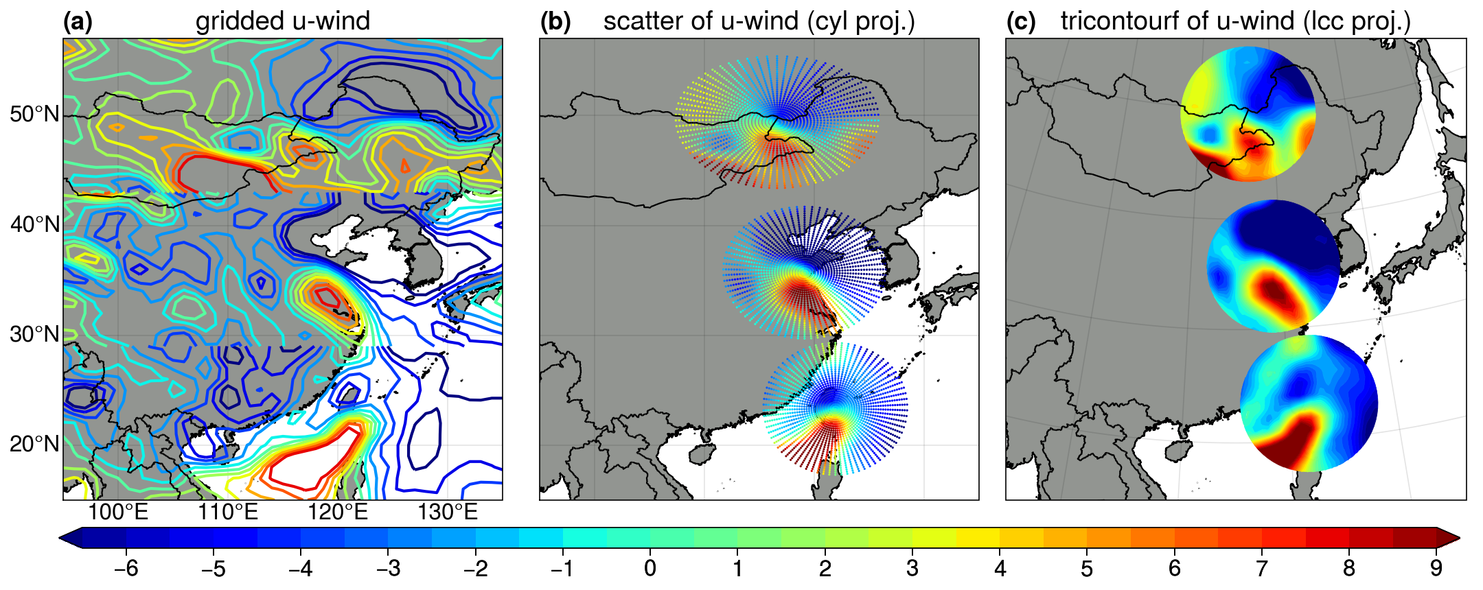
xvortices

1. Introduction

xvortices is a python package built on xarray (starts with an x), targeting at extracting information about moving vortices from lat/lon gridded datasets. Moving vortices include tornado, tropical cyclone, extratropical cyclone, polar vortex in the atmospheric context, as well as mesoscale eddy and ocean gyre in the oceanic context. These moving vortices are usually described in a moving (also known as quasi-Lagrangian) cylindrical coordinate. As the coordinate system moves on the spherical earth as a whole, one could take a view of the vortex dynamics from a quasi-Lagrangian perspective instead of the traditional Eulerian perspective.

Basically, this package would do the following jobs:

accept an xarray.Dataset (or a list of xarray.DataArray) as an input dataset, usually in a fashion of lat/lon grid;
interpolate the data onto the cylindrical coordinates once the origin of the moving coordinate is given (this is naturally done using the builtin function of xarray);
return the interpolated fields, including scalars and vectors;
re-project the vectors onto the azimuthal/radial directions;

With this tool, one can perform quasi-Lagrangian diagnoses of the structure, evolution, budget, intensity etc in a perspective different from the Eulerian one.

2. How to install

Requirements xvortices is developed under the environment with numpy (=version 1.15.4), xarray (=version 0.15.1), matplotlib (=version 3.4.3) and cartopy (=version 0.18.0). Older versions of these packages are not well tested.

Install from github

git clone https://github.com/miniufo/xvortices.git

3. Examples

3.1 A moving tropical cyclone

Here we demonstrate an application to the case of a moving tropical cyclone (TC) over the western North Pacific. One may need besttracks to load TC best-track data and cooperate with xvortices:

import xarray as xr
from xvortices import load_cylind, project_to_cylind

azimNum, radiNum, radMax = 72, 31, 6

# variables inside are [u, v, w, h]
dset = xr.open_dataset('gridded.nc')

# one can obtain tropical cyclone (TC) best-track
# data from the `besttracks` package
olon  = TC.get_as_xarray('lon') # timeseries of center longitudes
olat  = TC.get_as_xarray('lat') # timeseries of center latitudes
uovel = TC.get_as_xarray('uo')  # timeseries of center u-vel
vovel = TC.get_as_xarray('vo')  # timeseries of center v-vel

[u, v, w, h], lons, lats, etas = load_cylind(dset, olon=olon, olat=olat,
                                             azimNum=azimNum, radiNum=radiNum,
                                             radMax=radMax)
urel = u - uovel # storm-relative u
vrel = v - vorel # storm-relative v

# storm-relative azimuthal/radial winds
uaz, vra = project_to_cylind(urel, vrel, etas)

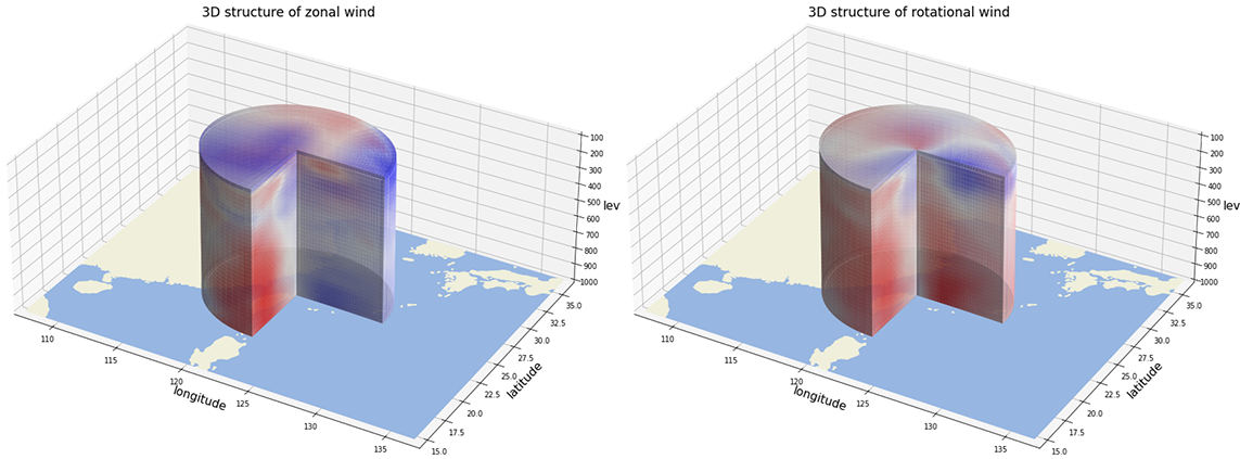
Plotting its 3D structure is also easy:

from xvortices import plot3D

# select the first time step to show
plot3D(lons[0], lats[0], uaz[0])

More details can be found at this TC notebook.

3.2 A moving mesoscale eddy

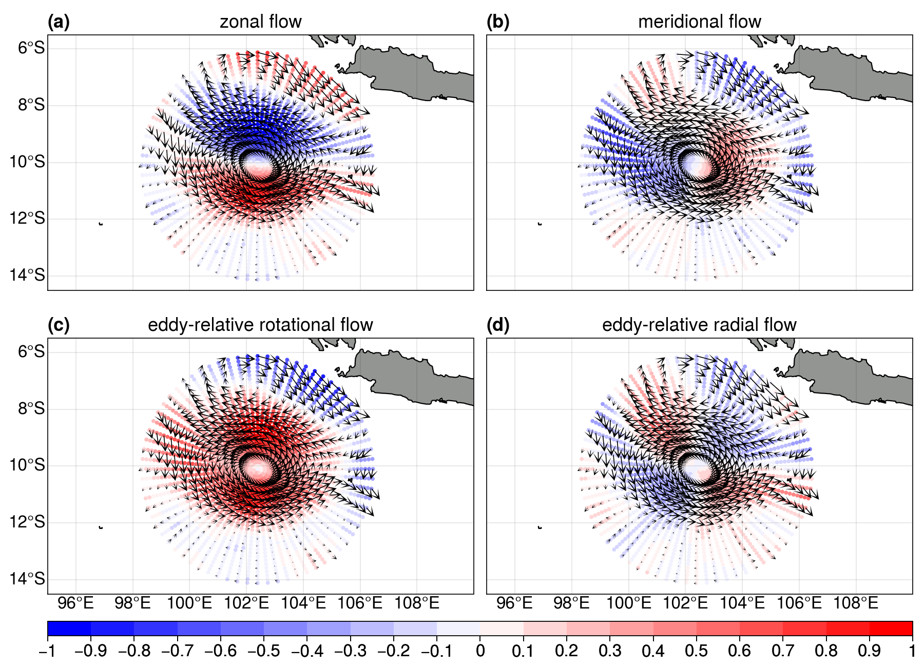
This is a mesoscale eddy case over the southern Indian Ocean.

import pandas as pd
import xarray as xr
from xvortices import load_cylind, project_to_cylind

# load an eddy positions from the "Mesoscale Eddy Trajectory Atlas" product
eddy = pd.read_csv('d:/SETIO2021.txt', sep='\s+', index_col='time', parse_dates=True)
# load AVISO gridded sea level anomaly and associated flow
dset = xr.open_dataset('D:/dataset-duacs-nrt-global-merged-allsat-phy-l4_SETIO_Eddy.nc')

# parameters of the cylindrical coordinates
azimNum, radiNum, radMax = 72, 31, 3

# interpolate from lat/lon grid to cylindrical grid
azimNum, radiNum, radMax = 72, 31, 4
[sla, adt, ugos, vgos], lons, lats, etas = load_cylind(dset[['sla','adt','ugos','vgos']],
                                             olon=eddy.lons.to_xarray(),
                                             olat=eddy.lats.to_xarray(),
                                             azimNum=azimNum, radiNum=radiNum,
                                             radMax=radMax,
                                             lonname='longitude',
                                             latname='latitude')

# calculate eddy's translating speed
uo = (eddy['lons'].diff()/86400*np.cos(np.deg2rad(eddy['lats']))).to_xarray()
vo = (eddy['lats'].diff()/86400).to_xarray()

# calculate eddy-relative current components
u_r = ugos - uo
v_r = vgos - vo

# project u/v to azimuthal/radial components
uaz, vra = project_to_cylind(u_r, v_r, etas)

More details can be found at this notebook.