R client for interacting with Google Cloud Natural Language APIs.
This is a work in progress. To date, this package only interacts with the analyzeSentiment API. If this project interests you, please let me know.
Google's documentation is fantastic. Click the link below for a quick start guide.
Before you can use Google's NLP APIs, you'll need an API key. For that, I recommend following the quick start guide linked above. It'll basically go something like this:
- Setup your Google software development account (Using the API is free up to a point, but you should be able to get a $300.00 credit for signing up as well). You may also need to "enable billing," but I promise that doesn't mean you're sinking any money into this thing--they clearly are trying to sell you on how awesome it is rather than tricking you into forking over cash.
- Enable the Natural Language API. There should be an option to "create credentials." For use in interactive R sessions, you'll just need an API key (a long string of text), which you should be able to get using the defaults provided by Google.
The first time you use any of the functions from the googleapis package, you'll be asked for your API key. It'll be set as an environment variable and saved for future sessions, so you should only have to do this once (per machine).
Install googleapis using the devtools package.
if (!"devtools" %in% installed.packages()) {
  install.packages("devtools")
}
devtools::install_github("mkearney/googleapis")Download tweets using the rtweet package, which can be installed from CRAN
install.package("rtweet")or the dev version from Github.
devtools::install_github("mkearney/rtweet")Use rtweet to download 1,000 non-retweeted Twitter statuses about Trump (for best results specify single language).
trump <- rtweet::search_tweets("Trump lang:en", n = 1000, include_rts = FALSE)Prep the text by first removing URLs, AT (@) mentions, and line breaks
trump_tweets <- gsub(
  "@\\S{1,}|http\\S{1,}|\\n", "", trump$text
)Second, because Google's sentiment analysis API will actually return sentiment scores for every sentence, remove any periods at the start of tweets.
trump_tweets <- gsub(
  "^\\.\\S{0,}", "", trump_tweets
)Third, remove all extra spaces (for the record, I'm not entirely sure if this matters, but if you're going to be analyzing individual words at any point, it's not a bad idea).
trump_tweets <- trimws(gsub(
  "[ ]{2,}", " ", trump_tweets
))
Here's what the tweets look like for me:
head(trump_tweets)## [1] "It's call respect for human life. We need to quit worshing things and get back to treating people like human beings."
## [2] "Trump bashing again tonight...#MAGA"
## [3] "Unfortunately we don't all get what we need but we get what we don't want.. that's Trump to ya"
## [4] "The snub was apparently in protest over the Trump administration's move to cut and delay aid to Egypt."
## [5] "Blimp (Trump) is the poster child for birth control! He's not even fit too be President of the PTA!"
## [6] "Nuts. Mexico always helps. Trump is guilty because he was ass to Mexico."
With the text ready to be analyzed, load googleapis if you haven't already.
library(googleapis)Conduct sentiment analysis on the character vector of tweets (text) using the analyze_sentiment() function.
sa <- analyze_sentiment(trump_tweets)Note: replicate this tutorial using the specific data set used here by reading in the R data files as done in the code below:
trump_tweets <- readRDS(
  "https://github.com/mkearney/googleapis/blob/master/data/text-trumptweets-demo.rds?raw=true"
)
sa <- readRDS(
  "https://github.com/mkearney/googleapis/blob/master/data/sa-trumptweets-demo.rds?raw=true"
)
The output is a bit messy, but it's easily converted into a tidy data frame using the as.data.frame or as_tibble functions.
sa <- tibble::as_tibble(sa)
sa
## # A tibble: 2,548 x 7
## id unit score magnitude position offset
## * <int> <chr> <dbl> <dbl> <int> <int>
## 1 1 document 0.0 0.9 NA NA
## 2 1 sentence 0.4 0.4 1 0
## 3 1 sentence -0.4 -0.4 2 34
## 4 2 document 0.0 0.0 NA NA
## 5 2 sentence 0.0 0.0 1 0
## 6 3 document -0.1 0.1 NA NA
## 7 3 sentence -0.1 -0.1 1 0
## 8 4 document -0.6 0.6 NA NA
## 9 4 sentence -0.6 -0.6 1 0
## 10 5 document 0.0 0.1 NA NA
## # ... with 2,538 more rows, and 1 more variables: content <chr>
Each row in the converted data frame represents one sentence of the provided text. For each observation, there are seven features (variables):
idID assigned to each document (in this case, each tweet)unitUnit of analysis, either "document" or "sentence"scoreThe sentiment (along positive and negative dimensions) score of the sentence standardized on a -1.0 to 1.0 scale.magnitudeThe magnitude of the score (positive, unstandardized)positionThe ordinal position of a given sentence as a sequence within a single tweet (e.g., first sentence of a document, second sentence of a document)offsetThe relative position, in number of characters, from which the sentence started within a documentcontentThe text that was analyzed (corresponds with unit)
Explore the data using the tidyverse.
## i subscribe to the tidyverse
suppressPackageStartupMessages(library(tidyverse))
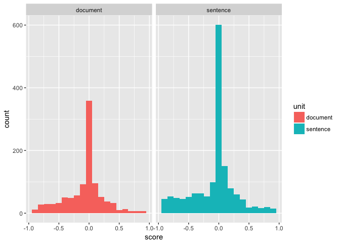
Histogram of scores faceted by unit
sa %>%
  ggplot(aes(score, fill = unit)) +
  geom_histogram(binwidth = .1) +
  facet_wrap(~ unit)
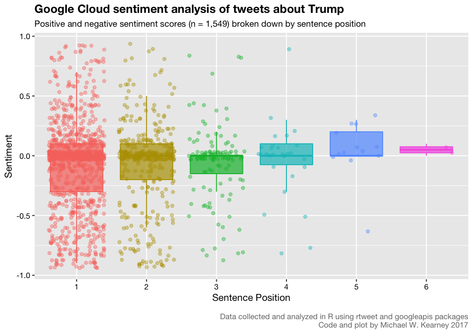
Box plot for each sentence position number
p <- sa %>%
  filter(unit == "sentence") %>%
  mutate(position = factor(position)) %>%
  ggplot(
    aes(x = position, y = score, colour = position, fill = position)
  ) +
  geom_boxplot(outlier.shape = NA, alpha = .7) +
  geom_jitter(alpha = .4, shape = 21) +
  theme(
    legend.position = "none",
    text = element_text(family = "Helvetica Neue", colour = "black"),
    axis.text = element_text(colour = "black"),
    plot.caption = element_text(size = rel(.8), colour = "#777777"),
    plot.title = element_text(face = "bold")
  ) +
  labs(
    title = "Google Cloud sentiment analysis of tweets about Trump",
    subtitle = "Positive and negative sentiment scores (n = 1,549) broken down by sentence position",
    x = "Sentence Position",
    y = "Sentiment",
    caption = "\nData collected and analyzed in R using rtweet and googleapis packages\nCode and plot by Michael W. Kearney 2017"
  )

png("demo_plot.png", 7.5, 5.3, "in", 10, res = 127.5)
p
dev.off()
