FMoW: The Functional Map of the World Dataset

These are my notes on getting started with fMoW.

Most of this info is from the fMoW paper: arxiv:1711.07846
For download instructions see the github.com/fMoW/dataset#download
For citing fMoW see github.com/fMoW/dataset#references

Quick start

For an easy ImageFolder-compatible version of fMoW, use the create_msrgb_imagefolder.py script:

python create_msrgb_imagefolder.py --data_dir <path_to_fmow> --dst_dir <path_to_new_dst>

This version has the following stats:

Num train images: 363572
Num val images: 53040

Pixel mean:  tensor([0.3791, 0.3804, 0.3546])
Pixel std:  tensor([0.2622, 0.2549, 0.2561])

Folder structure

The fMoW folder structure almost adheres to the PyTorch ImageFolder format, but not quite. Within each class folder there are subfolders that each correspond to a particular location - as in, a location on the Earth where a structure/facility of the respective category is present. Each of these subfolders holds many images and metadata for its particular location taken at different times e.g. ~months apart. The overall folder structure is depicted below:

fMoW
    \
     |-- train
     |        \
     |         |-- class1
     |         |         \
     |         |          |-- class1_0
     |         |          |           \
     |         |          |            |-- class1_0_0_msrgb.jpg
     |         |          |            |-- class1_0_0_msrgb.json
     |         |          |            |-- class1_0_0_rgb.jpg
     |         |          |            |-- class1_0_0_rgb.json
     |         |          |            |-- ...
     |         |          |            |-- class1_0_<n>_msrgb.jpg
     |         |          |            |-- class1_0_<n>_msrgb.json
     |         |          |            |-- class1_0_<n>_rgb.jpg
     |         |          |            |-- class1_0_<n>_rgb.json
     |         |          |-- ...
     |         |          |-- class1_<n>
     |         |-- ...
     |         |-- class<n>
     |-- val
            \
             |-- class1
             |-- ...
             |-- class<n>

As an example, the first class in alphabetical order is "airport" and within the airport train folder, there are 463 locations:

fMoW
    \
     |-- train
     |        \
     |         |-- airport
     |         |          \
     |         |           |-- airport_0
     |         |           |-- ...
     |         |           |-- airport_462

Within the first location, airport_0, we see that there are 8 temporal views (0 ... 7):

|-- airport
           \
            |-- airport_0
                         \
                          |-- airport_0_0_msrgb.jpg
                          |-- airport_0_0_msrgb.json
                          |-- airport_0_0_rgb.jpg
                          |-- airport_0_0_rgb.json
                          |-- ...
                          |-- airport_0_7_msrgb.jpg
                          |-- airport_0_7_msrgb.json
                          |-- airport_0_7_rgb.jpg
                          |-- airport_0_7_rgb.json

Notice that there are 4 files for each view: two types of images, each with a dedicated json metadata file. Let's start with the two image types msrgb and rgb:

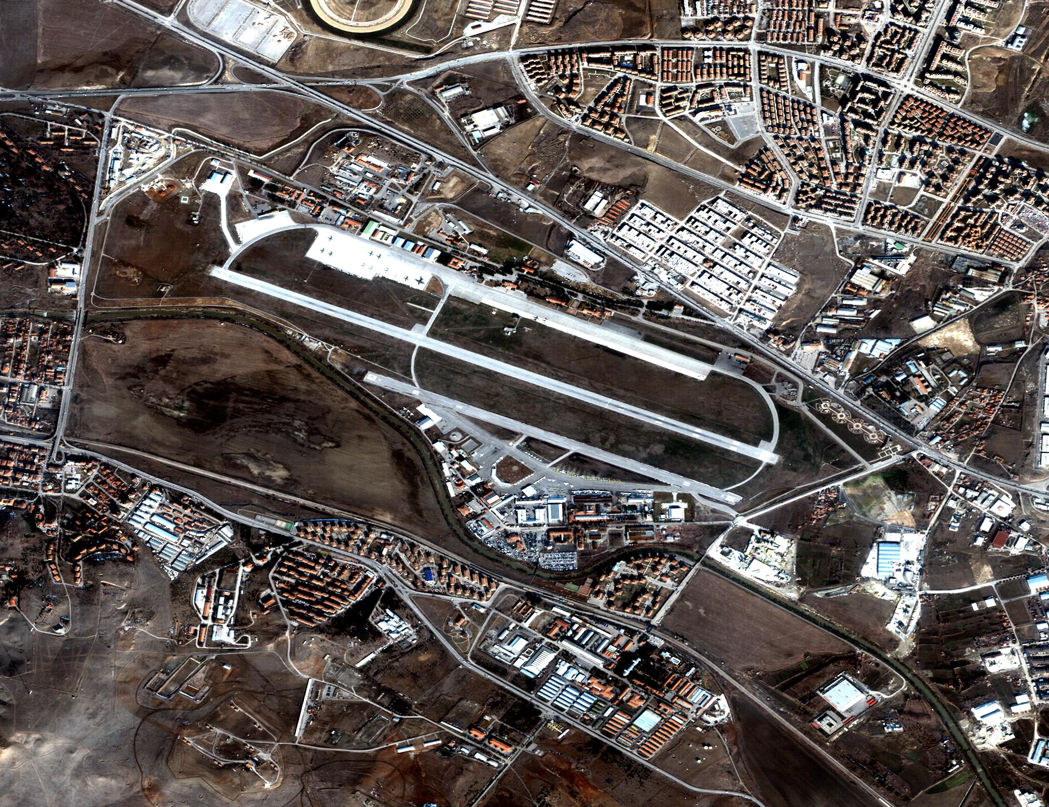
msrgb: This format results from extracting the red, green, and blue channels from a multispectral (ms) image which originally contained either 4 or 8 channels in total. The extra channels correspond to different wavelengths of light both in the visible spectrum and "near-infrared" (NIR):

img src: Maxar blog post on MSI

Here is the msrgb image airport_0_0_msrgb.jpg:
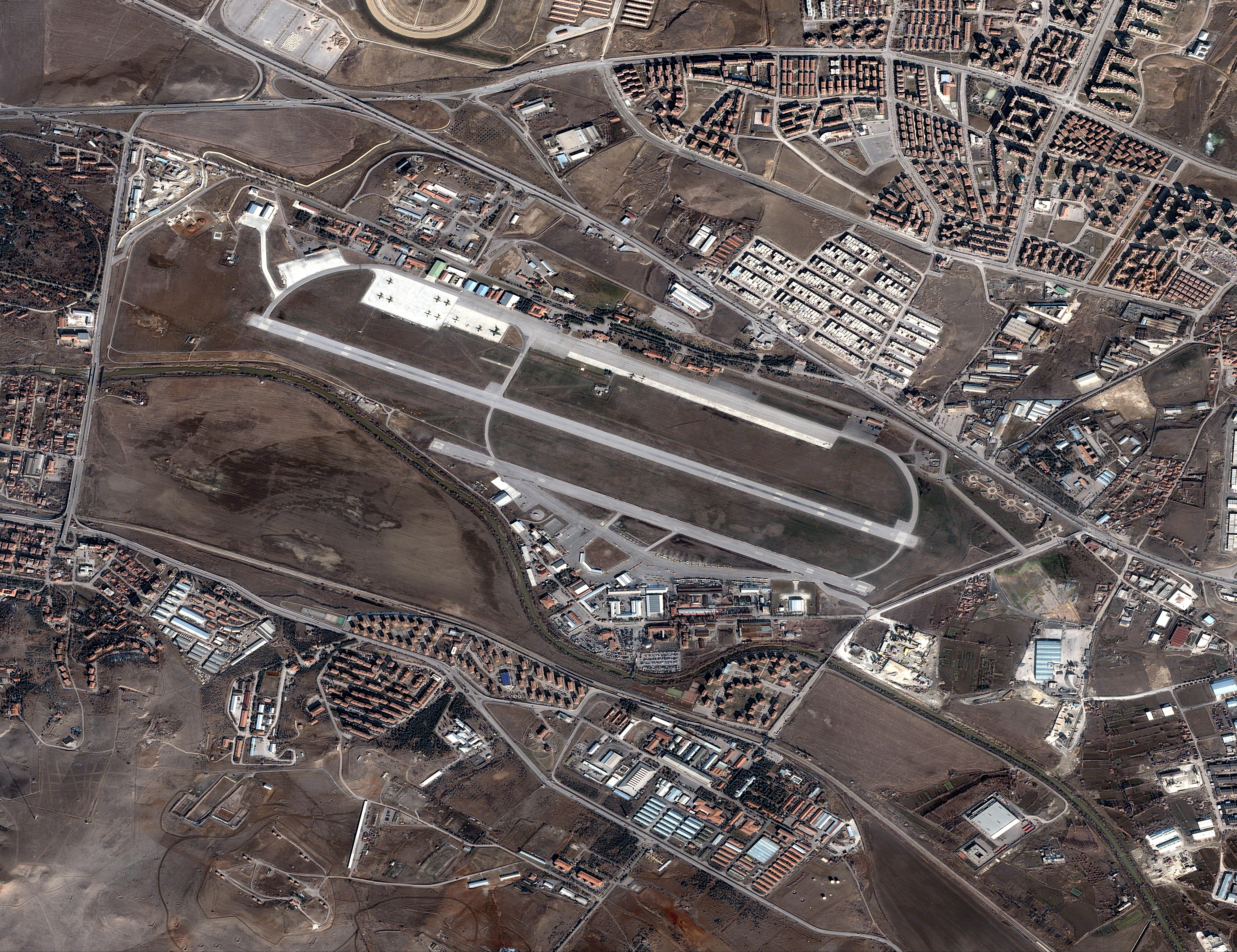
rgb: This format combines the rgb data with a panchromatic image (i.e. single-channel a.k.a grayscale) that was taken simultaneously at a much higher resolution. The merging of the two resolutions happens through an image processing technique called pan-sharpening. The result is a high-res, color image

img src: Maxar blog post on MSI

Here is the pan-sharpened rgb image airport_0_0_rgb.jpg:
- In terms of visual appearance, we can see that the pan-sharpening process yields a sharper image with less saturated colors.
- The big difference is the resolution (image size). This pan-sharpened rgb image is 8200 x 6312 pixels, whereas the msrgb image is 2050 x 1578

fMoW stats

Temporal views

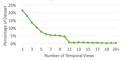
As mentioned above, each location in each class has multiple images taken at different times. The fMoW paper refers to these as "temporal views". To answer the question, "how many temporal views does each location (area) have?", the paper provides a plot of the distribution:

Looking at this, we could say most of the dataset has 5 or less views. It is noted in the paper that the max number of views for any single area is 41.

Instances per class

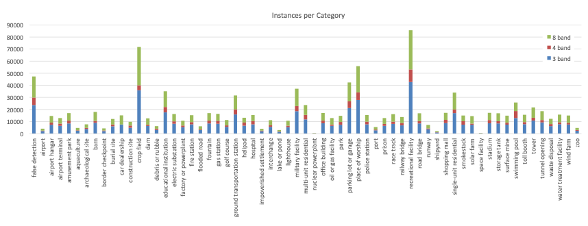
The total instances per class are unevenly distributed: