mleonowicz/3DJigsawSolver

3D Jigsaw Solver - Report

Problem definition

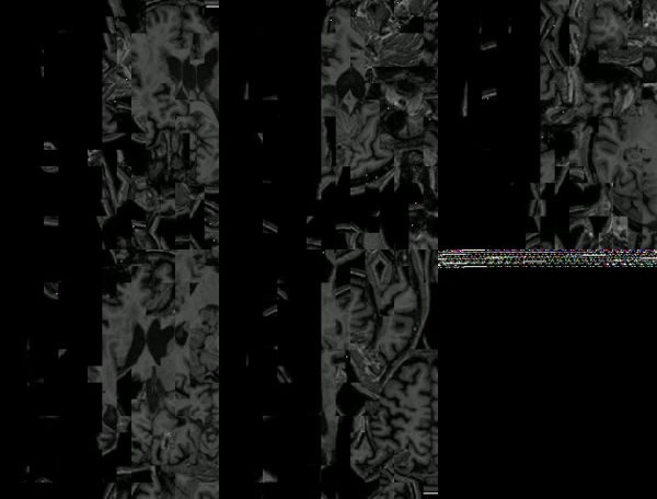
In our project, we use a genetic algorithm to solve the jigsaw puzzle problem. In the paper, the method was shown for solving 2D puzzles. We are generalizing the solution for the 3D case.

We have $n$ three-dimensional puzzle pieces that are constructed by splitting the input video/3D image. The goal is to reconstruct the original input by exploring the space of possible puzzle permutations without any information about the original puzzle.

Used paper - https://arxiv.org/pdf/1711.06767.pdf

Our implementation is based on a paper that proposes a solution for 2D puzzles. We expand on the ideas introduced there.

Implementation

We take the input - either a 3D image; or a video (in that case the time will be considered as the third dimension). We split it into $n$ identically shaped puzzles to form a puzzle of $W \times H \times Z$ shape. We then follow the genetic algorithm of the form:

• Create an initial population - each individual has randomly placed puzzle pieces.
• For each generation:
  • Evaluate the current population using the fitness function.
  • Pick $N_E$ elites that remain in the population.
  • Randomly choose (with weights based on fitness values) two members of the population and apply the crossover operator to them to create a new offspring. With $\beta$ probability perform mutation in a procedure described below. Repeat that until the population is full.
• Return the puzzle solution with the best fitness score.

Fitness

We define the dissimilarity function between two puzzle pieces $x_i$ and $x_j$, where $x_i, x_j$ are of size $W \times H \times Z$. Let's assume, that the pieces are in front-back relation, i.e. $x_j$ is the backward piece and $x_i$ is the frontal one. Their dissimilarity (considering this front-back relation) $D_Z$ is calculated as follows:

$$D_Z(x_i, x_j, r) = \sqrt{\sum_{w=1}^W \sum_{h=1}^H \sum_{c=1}^3 (x_i(w, h, Z, c) - x_j(w, h, 1, c))^2}$$

$D_H, D_W$ are dissimilarity functions for the up-down and left-right directions respectively and are defined in the same way.

Intuitively, we calculate the difference between adjacent borders of two pieces (in RGB format) that are next to each other. It is based on the premise, that adjacent pieces in the original puzzle should share similar border coloring.

The fitness function of the entire puzzle solution is the sum over dissimilarity measures between all pairs of neighbor pieces in all three directions.

Crossover

During the crossover operation, we maintain a kernel - a set of pieces with relative positions saved. We add new pieces to the kernel iteratively by taking the best-fit piece for the current configuration in a greedy manner. The exact position of each piece is set at the final step of the kernel creation; when all puzzle pieces are added into the kernel. The intuition behind the operation is that when adding a new piece to the kernel it should be possible to shift around 'the board'. We do not want to fix the puzzle piece into a single position, but rather we place the piece based on its position relative to other pieces.

Crossover operator definition:

• Start by adding a random piece to the kernel
• Every time a new puzzle is added, check each of its borders that are not occupied (left, right, up, down, forward, backward) and for each of those borders calculate which piece is the best fit for that place using the following steps.
  • If both parents have the same puzzle adjacent to the piece under consideration and this puzzle is in the available pieces it is used and added to the kernel.
  • If the added puzzle has a best-buddy puzzle in the available piece and it is an adjacent puzzle in at least one of the parents then it is added to the kernel.
  • A puzzle that is the best fitting puzzle from the available pieces is added to the kernel.

Pieces $P_1$ and $P_2$ are best-buddy pieces if for one of $P_1$'s borders, $P_2$ has the smallest dissimilarity, and for the corresponding border of $P_2$ the best fit is $P_1$.

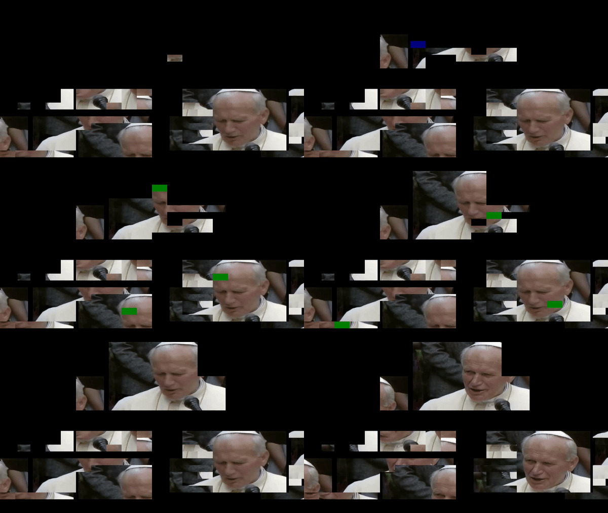
In the visualization video, the bottom two puzzles represent the parents that are picked to create a new offspring. The upper puzzle is the new offspring. New pieces are added iteratively. The green color means that both of the parents agreed on that piece. Blue color means that the best-buddy puzzle was picked.

Mutation

We introduce two types of mutations:

• In the crossover operator when calculating the best-fit puzzle a randomly chosen puzzle from the available pieces is picked and added to the kernel instead with probability $\alpha$.
• After the crossover operator with probability $\beta$ a mutation is performed by reversing the order of the puzzle placement in the third dimension (depth). Let's consider layers of puzzle pieces, placed along the third dimension. Two indices are picked $0 \leq i \leq j \leq Z$ and then puzzle layers between the $i$ and $j$ are inversed. For example, if $i = 2$ and $j = 5$ then pieces of depth $2$ swap with pieces of depth $5$ and pieces with depth $3$ swap with pieces of depth $4$.

Results

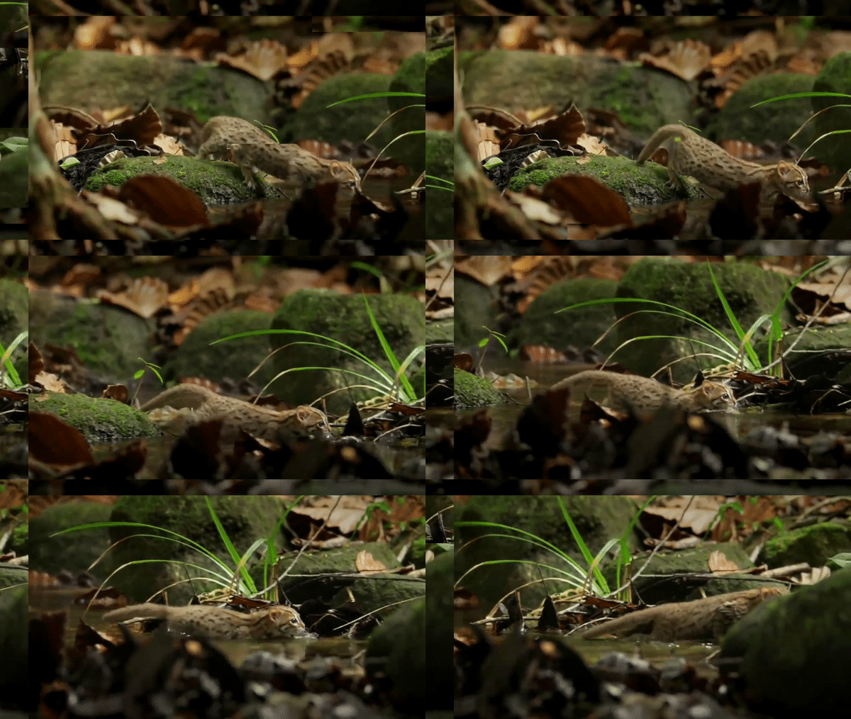
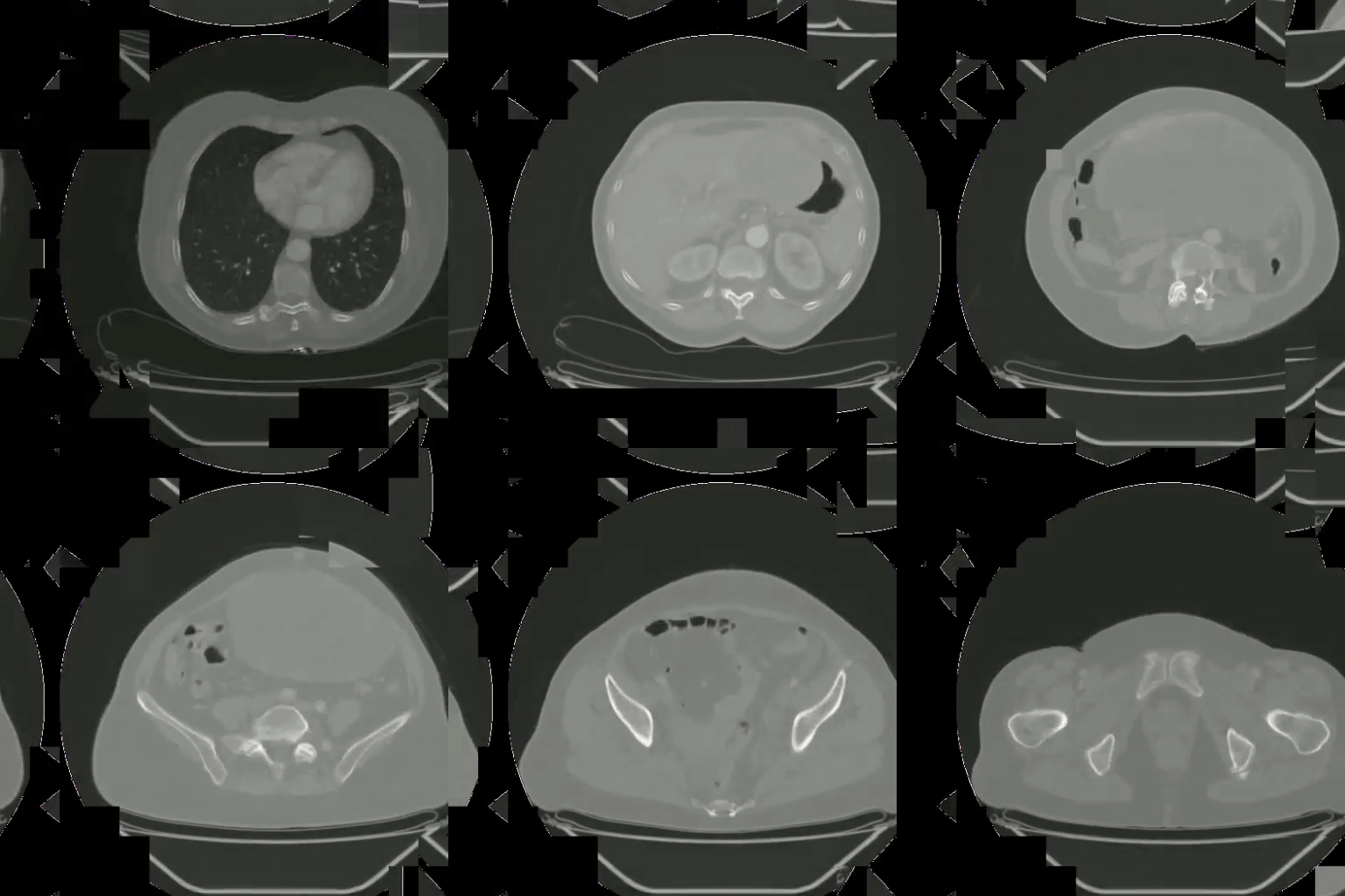
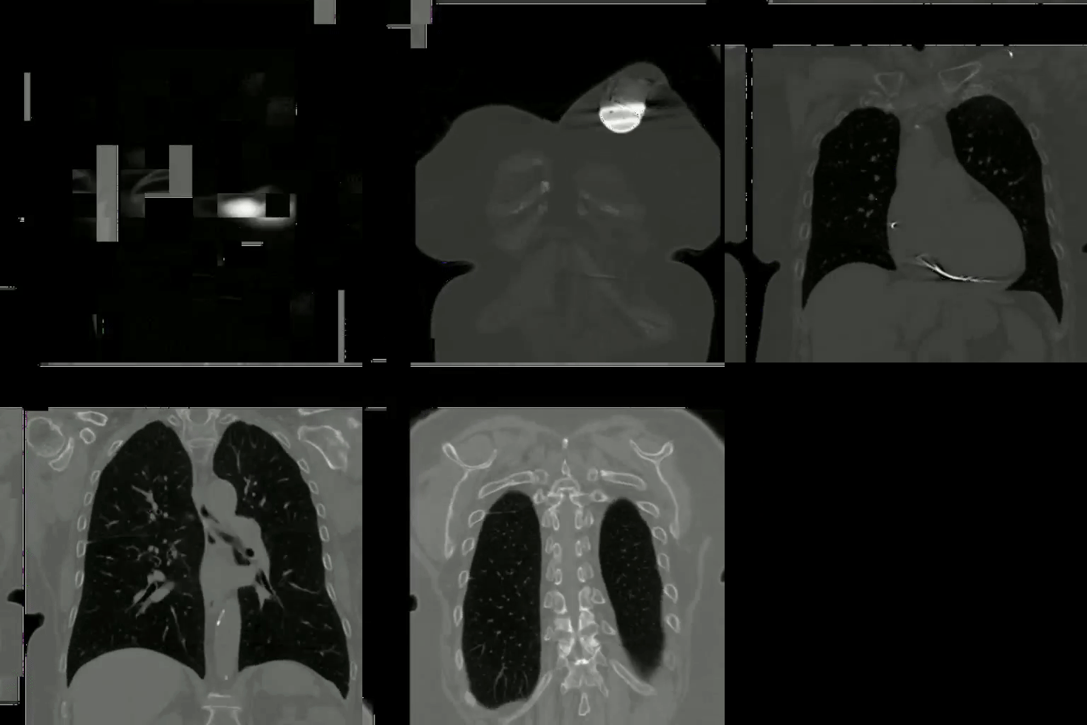
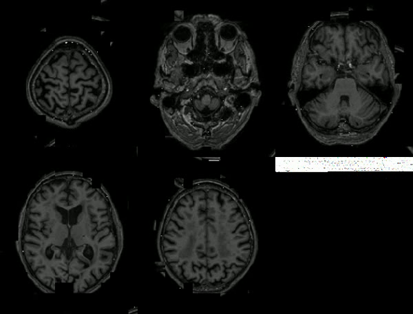
We have tested the image on two youtube videos and three 3D images of medical scans.

Each experiment was run with the following parameters:

• Population number: 500
• Number of puzzles: 3375 - $15 \times 15 \times 15$ puzzles in each dimension
• Number of elites: 15
• $\alpha$: 0.003
• $\beta$: 0.05
• Maximum number of generations: 100

Results for each image:

Video no. 1

To run this example use:

python3 main.py --video-path example/example.mp4

Video no. 2

To run this example use:

python3 main.py --video-path example/example2.mp4

3D Image no. 1

To run this example use:

python3 main.py --video-path example/scan-1.avi

3D Image no. 2

To run this example use:

python3 main.py --video-path example/scan-2.avi

3D Image no. 3

To run this example use:

python3 main.py --video-path example/brain_scan.nii.gz --input-type image

Ablation study

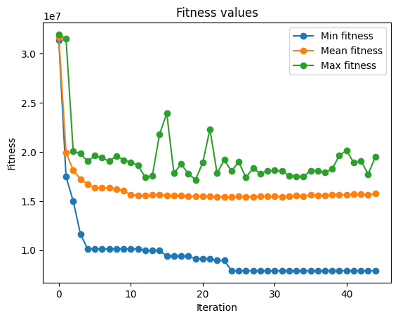
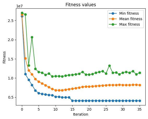
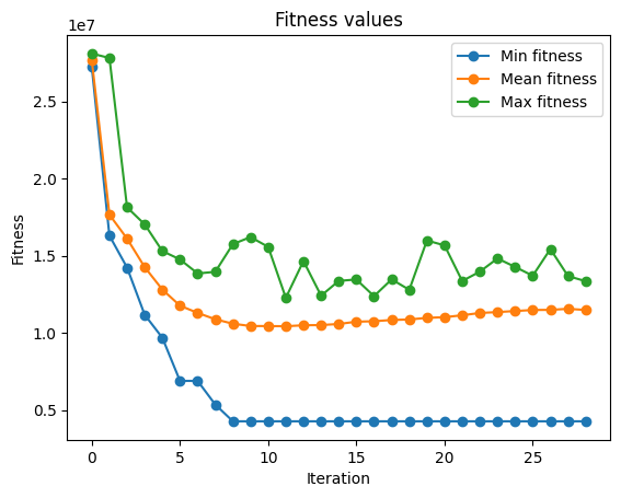
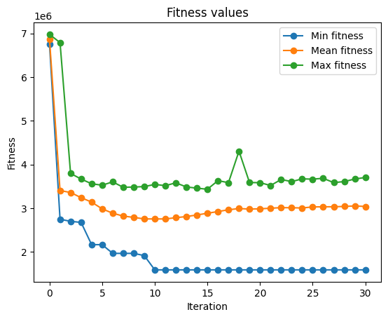
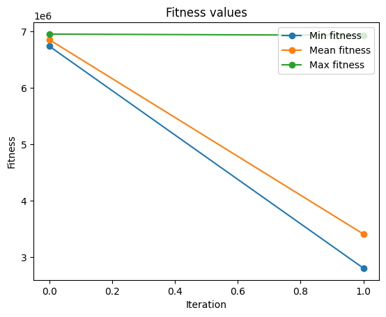
As we can see from the results, the presented algorithm finds the best solution in a matter of a couple of generations. Most notably, the crossover operation as it is defined right now is quite powerful. We have performed the ablation study to analyze the power of this operation.

At first, we analyzed less sophisticated crossover operation that instead performs only two steps:

• If both parents have the same puzzle adjacent to the piece under consideration and this puzzle is in the available pieces it is used and added to the kernel.
• Add a random piece at the considered position to the kernel.

The results can be seen here:

Hyperparameters used:

• Population number: 500
• Number of puzzles: 3375 - $15 \times 15 \times 15$ puzzles in each dimension
• Number of elites: 15
• $\alpha$: 0.003
• $\beta$: 0.05
• Maximum number of generations: 100

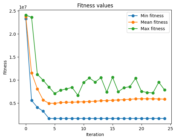
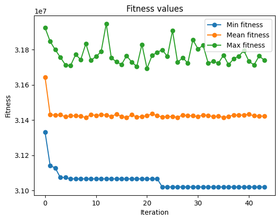
As presented above, this model has not enough power to produce satisfactory results.

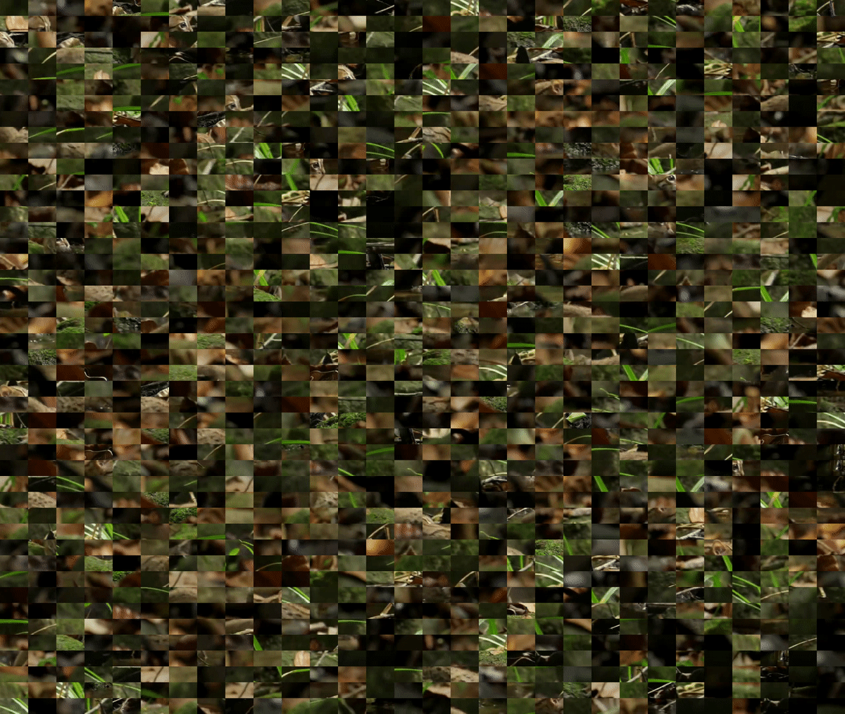
The other thing that we have checked is whether the evolution mechanism adds anything to the algorithm at all. We have tried finding a solution for the same inputs, running the algorithm for a single generation, so that we are spanning the crossover across the entire population only once. The results of the experiment are as follows:

Hyperparameters used:

• Population number: 500
• Number of puzzles: 3375 - $15 \times 15 \times 15$ puzzles in each dimension
• Number of elites: 15
• $\alpha$: 0.003
• $\beta$: 0.05
• Maximum number of generations: 1

As seen in the example, the results are better than a randomly generated puzzle; but still lack general cohesion.

Further Work

• As can be seen in the examples provided as the evolution goes on, at some point, the mean of population fitness slightly increases. This is an unexpected behavior, one that would require a thorough investigation.
• We have seen a significant increase in puzzle solution accuracy after introducing the $\beta$ parameter and related mutation procedure. One can experiment with such mutation to see what would work the best (for example - a more general form, considering layers from all dimensions instead of only the depth of the puzzle).
• Create new metrics so that the performance of the model can be measured more accurately. Those metrics would be used to calculate how good is the final best individual compared to the optimal solution.
• Create a new fitness function. As seen in the examples dissimilarity is not an optimal choice for this problem. For some puzzles, it is possible to find an individual that has a better fitness score than the best solution.

Sources:

Medical scans

World's smallest cat 🐈

Pytania do Jana Pawła II