This repository is the official implementation of Linear Connectivity Reveals Generalization Strategies.
To install requirements:
bash install_basics.shTo download and assign labels to PAWS-QQP dataset for evaluation:
bash get_paws.shTo fine-tune a QQP model, using the original script, we run the following commands.
First, we fetch the pre-trained weights:
cd finetune/bert
wget https://storage.googleapis.com/bert_models/2018_10_18/uncased_L-12_H-768_A-12.zip
unzip uncased_L-12_H-768_A-12.zip
Then, we downgrade environment to meet requirements of Google's bert fine-tuning script:
conda install python=3.7
conda install tensorflow-gpu==1.15.0
pip install numpy==1.19.5
Next, download and prepare QQP data:
pip install getgist
getgist raffaem download_glue_data.py
python3 download_glue_data.py --data_dir glue_data --tasks QQP
Finally, train the model:
export BERT_BASE_DIR=./uncased_L-12_H-768_A-12
export GLUE_DIR=./glue_data
export MODEL_NUM=0

python3 run_classifier.py \
  --task_name=qqp \
  --do_train=true \
  --do_eval=true \
  --data_dir=$GLUE_DIR/QQP \
  --vocab_file=$BERT_BASE_DIR/vocab.txt \
  --bert_config_file=$BERT_BASE_DIR/bert_config.json \
  --init_checkpoint=$BERT_BASE_DIR/bert_model.ckpt \
  --max_seq_length=128 \
  --train_batch_size=32 \
  --learning_rate=2e-5 \
  --num_train_epochs=3.0 \
  --output_dir=qqp_save_$MODEL_NUM --save_checkpoints_steps=5000
Next, we delete the environment and recreate another for updated version of packages:
conda deactivate
rm -rf ./ext3
bash install_basics.sh
After the training has completed, to convert the model weights to PyTorch and upload them to HuggingFace-Hub, we can do the following:
python3 convert_to_pt.py $MODEL_NUM <hf_auth_token>where <hf_auth_token> is a HuggingFace AuthToken with WRITE permissions.
The following command can be used to train the CoLA models, using this HuggingFace script.
cd cola/
export TRAINING_SEED=0
python run_flax_glue.py \
        --model_name_or_path bert-base-uncased\
        --task_name cola \
        --max_seq_length 512 \
        --learning_rate 2e-5 \
        --num_train_epochs 6 \
        --per_device_train_batch_size 32 \
        --eval_steps 100 --save_steps 100\
        --output_dir bert-base-uncased_cola_ft-$TRAINING_SEED/ \
        --seed $TRAINING_SEED --push_to_hub --hub_token <hf_auth_token>
Each finetuning run must be given a different seed.
All the following steps assume that the finetuned models are available on HuggingFace-Hub.
All our finetuned models, along with MNLI models finetuned by McCoy et. al. 2019, are available on HuggingFace-Hub here.
Additionally, the repository of each model contains the sample-wise logits, predictions and labels for all the evaluation datasets used for that model in json files.
We provide a Colab Notebook which can be used for running all the following sections.
To evaluate a model, run:
cd evaluate/glue
python3 eval_models.py --base_models_prefix connectivity/bert_ft_qqp- --dataset paws --split dev_and_test --models 0 1 2 3\
                       --write_file_prefix eval_qqp-
For a complete list of all available options and their use, run python3 eval_models.py -h. To upload an evaluation file to HuggingFace-Hub, you can run:
python3 push_to_hub.py <REPO_NAME> <FILE> <AUTH_TOKEN> [<PATH_IN_REPO>]The fourth argument is optional and specifies the path in repository where <FILE> will be stored.
To interpolate between pairs of models, run:
cd interpolate
python3 interpolate_1d.py --base_models_prefix connectivity/bert_ft_qqp- --dataset qqp --split validation\
                          --save_file interpol.pkl --suffix_pairs 7,22 7,98 22,98 1,7 1,98 > output.log
For a complete list of all available options and their use, run python3 interpolate_1d.py -h.
To get the loss values on a 2-D plane containing three models, run:
cd interpolate
python3 interpolate_2d.py --base_models_prefix connectivity/feather_berts_ --anchor 99 --base1 44 --base2 87\
                          --dataset hans --split test --metric ECE > output.log
The above command will calculate values for plottting the HANS-LO loss, accuracy and ECE surfaces on the plane containing model number 99, 44 and 87 from the Feather-BERTs. For a complete list of all available options and their use, run python3 interpolate_2d.py -h.
To compute the
cd misc/
python3 measure_flatness.py --model connectivity/feather_berts_0 --n_batches 8192
For a complete list of hyperparameters and their usage, run python3 measure_flatness.py -h. In particular, you can specifyt he --epsilon <val>.
Additionally, you can also specify the number of directions in which to optimize(the --num_random_dirs <p>.
You can use your own interpolation and evaluation logs. Or fetch our logs from HuggingFace-Hub into a directory as follows.
mkdir logs/
python3 get_logs.py logs/
rm  logs/*.lock
To get the inteprolation logs, simply run:
cd logs
git clone https://huggingface.co/connectivity/interpolation_logs/cd plot/
sufs="";for i in {0..99}; do sufs="$sufs $i";done;
python3 peak_valley_plains.py --perf_metric lexical_overlap_onlyNonEntailing --interpol_datasets MNLI\
--interpol_log_dirs ../logs/interpolation_logs/mnli_interpol@36813steps/\
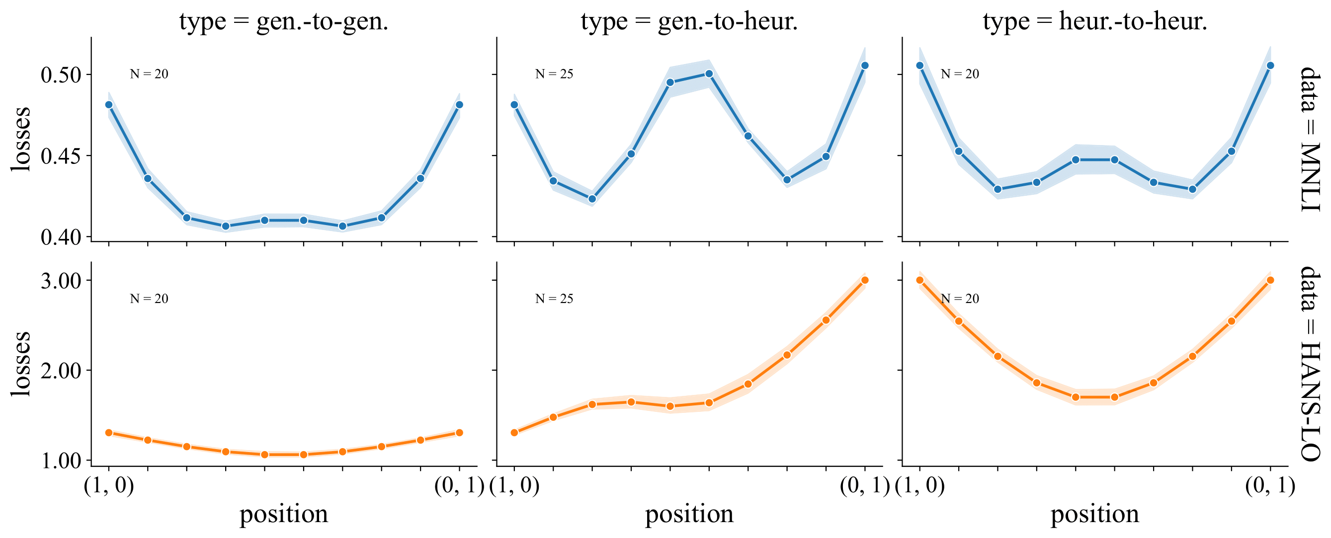
--eval_mods_prefix ../logs/hans_eval_bert_ --eval_mods_suffixes $sufs --remove_plainsThe above command finds 5 lowest, 5 highest and 5 intermediate performing models on lexical_overlap_onlyNonEntailing samples, by reading the evaluation logs from the files specified by --eval_mods_prefix and --eval_mods_suffixes.
The interpolations are read from the directory specified in --interpol_log_dirs, and the interpolations between the highest(generalizing) and lowest(heuristic) performing models are plotted.
The --remove_plains option omits plotting interpolations between intermediate models, and the heuristic and generalizing models.
cd /content/connectivity_gems/plot/
export BASE_DIR=../logs/interpolation_logs/interpol_2d/short_range
python3 same_z_scale_plot.py --surface_pkl_files $BASE_DIR/around_peaks/mnli_test/mnli_test_99_8_37_2_loss_surface.pkl\
                                                 $BASE_DIR/around_valleys/mnli_test/mnli_test_44_73_89_2_loss_surface.pkl\
                                                 $BASE_DIR/peak_and_2valleys/mnli_test/mnli_test_99_44_73_2_loss_surface.pkl\
                              --plot_title "" --names '(a.) generalized models' '(b.) heuristic models'\
                                                      '(c.) generalized and heuristic models' \
                              --point_names G0 G1 G2 H0 H1 H2 G0 H0 H1 --clip_x -0.5 1.5 --clip_y -1.0 1.20 --clip_z 0 0.65
The above command plots the three loss surfaces specified in --surface_pkl_files with same color scale. --clip_x, --clip_y, --clip_z specify the range for
cd plot
sufs="";for i in {0..99}; do sufs="$sufs $i";done;
python3 interpol_heatmap.py --order_by perf --eval_metric f1 \
                    --interpol_log_dir ../logs/interpolation_logs/qqp_interpol@34110steps/ \
                    --eval_mods_prefix ../logs/paws_eval@34110steps_bert_ft_qqp-\
                    --eval_mods_suffixes $sufs --emb_acc_corr --ticks accs
The --order_by flag specifies which quantity to use to order the model on the axes of the heatmap. It can be one of [seed, perf, cluster]. In the above command, models will be ordered in increasing order of performance.
The --eval_metric specifies which metric to use to calculate performance of a model. It can be one of [loss, accuracy, f1, matthews_correlation] depending on what metrics are available for the dataset in HuggingFace metrics(See here).
The --emb_acc_corr, when passed, will generate a scatter plot relating the cluster membership and performance of the models.
The --ticks flag is used to specify what ticks to display on the axes of the heatmap and can be one of [seed, accs]. Using --ticks accs will display performance values on the axes.
For complete details run the script with -h flag, as before.
cd plot
sufs="";for i in {0..99}; do sufs="$sufs $i";done;
export BASE_DIR=../logs/interpolation_logs/qqp_interpol@
python3 dynamics.py --eval_metric f1 --interpol_log_dirs ${BASE_DIR}15000steps/ ${BASE_DIR}25000steps ${BASE_DIR}34110steps \
                    --eval_mods_prefixes ../logs/paws_eval@34110steps_bert_ft_qqp- ../logs/paws_eval@34110steps_bert_ft_qqp-\
                    ../logs/paws_eval@34110steps_bert_ft_qqp- --eval_mods_suffixes $sufs
The above command will plot the change in cluster membership with training. For complete details run the script with -h flag, as before.
Some of the code in src/constellations/simplexes is borrowed from this work. And the google script has been modified from this repo.
