geodetic_inversion

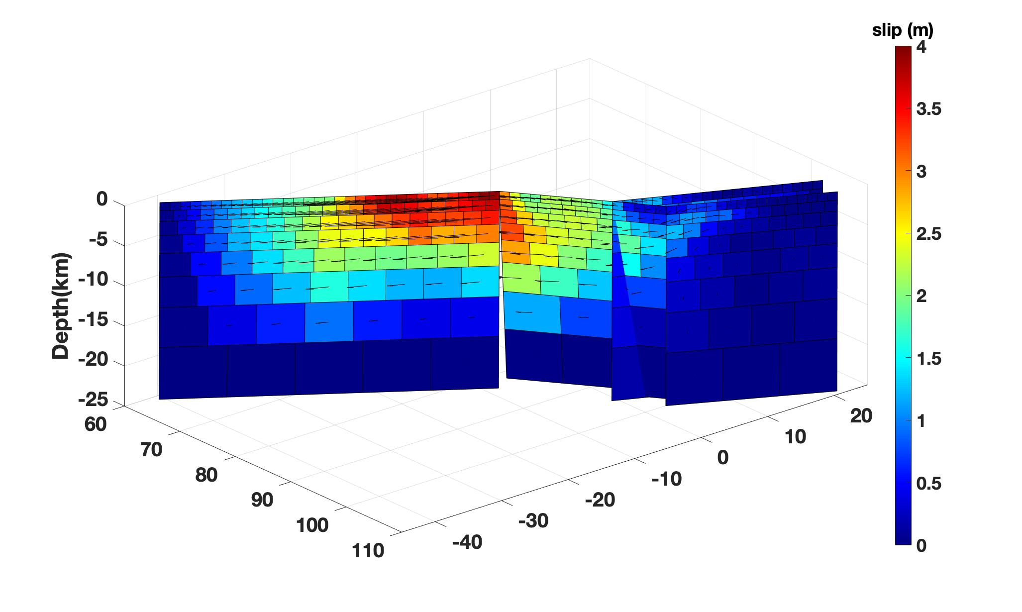
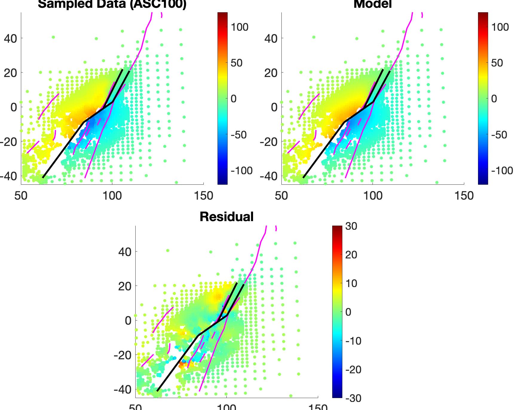
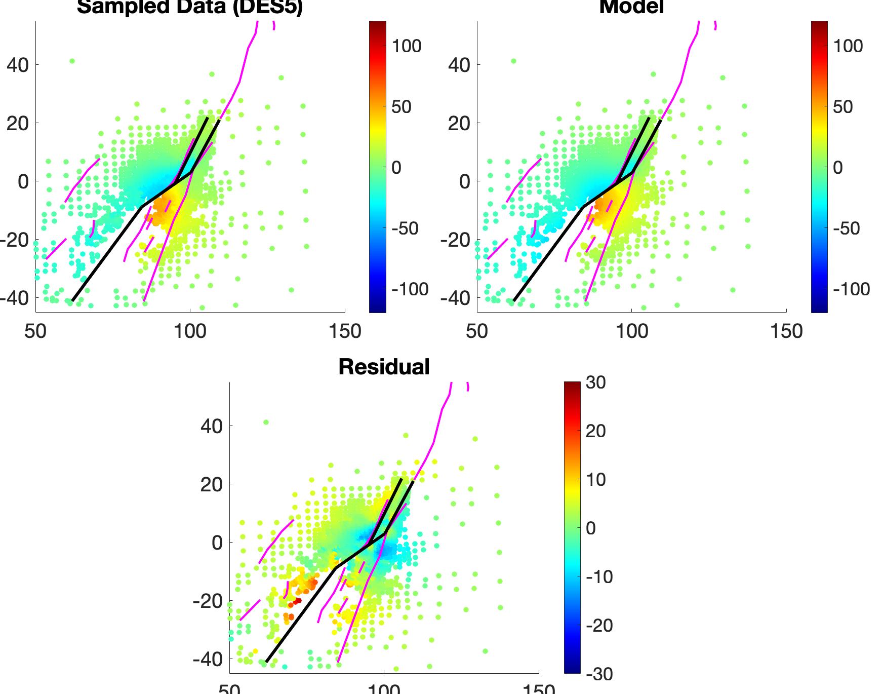
This repo homogeneous/layered inversion using InSAR/GPS

New: currently the repo also supports non-linear fault construction and inversion!

References:

(Please cite those works if using our codes)

Jin, Z., & Fialko, Y. (2020). Finite slip models of the 2019 Ridgecrest earthquake sequence constrained by space geodetic data and aftershock locations. Bull. Seism. Soc. Am., 110, 1660–1679.

Jin, Z., & Fialko, Y. (2021). Coseismic and early postseismic deformation due to the 2021 M7. 4 Maduo (China) earthquake. Geophysical Research Letters, 48(21), e2021GL095213.

Jia, Z., Jin, Z., Marchandon, M., Ulrich, T., Gabriel, A. A., Fan, W., ... & Fialko, Y. (2023). The complex dynamics of the 2023 Kahramanmaraş, Turkey, M w 7.8-7.7 earthquake doublet. Science, 381(6661), 985-990.

Jin, Z., Fialko, Y., Yang, H., & Li, Y. (2023). Transient deformation excited by the 2021 M7. 4 Maduo (China) earthquake: Evidence of a deep shear zone. Journal of Geophysical Research: Solid Earth, 128(8), e2023JB026643.

Step 1 ~ 2 are written in the file `main_detrend_inversion.m`

Step 0: setup your MATLAB, CSHELL and GMT paths.

Please include the MATLABPATH for all directories.

Step 1: data cleaning using `clean_insar_data.m`

% remove some near-field unwrapping errors manually first
clean_insar_data;

If you open clean_insar_data.m, you need to specify following information to clean the data:

this_track: the directory that InSAR grid file is saved.
insar_file = 'unwrap_ll.grd': the interferogram/offsets grid
mask_file = 'mask_txt': the masking TXT file that writes the masking polygon files (e.g. mask1.txt, mask2.txt, ...). The masking polygons could be generated using Google Earth KML files.

Then the subroutine runs as (inside clean_insar_data.m):

% scale = -lambda / 4 / pi
% scale = -4*pi if the insar_file is an offset grid
% los_max is used just for plot (cm)
% detrend = 1 means that you apply for a detrend with the topography
mask_insar_phase(this_track, insar_file, mask_file, scale, 'los_max', 80, 'detrend', 0);

This step would output a subsampled grid file called "unwrap_clean_sample.grd", in 100 meters resolution as default.

Step 2: detrend the phase and remove the phase ambiguity

If we have enough far-field GPS data, we could use those GPS data to invert a coarse slip model to detrend the unwrapped phase.
In cases such as Pamir and Qinghai earthquake, since we do not have enough GPS sites covered, we could just assume a far-field pixel that corresponds to zero displacement.

% grdin = '/Users/zej011/coseismic/DES5/LOS2/unwrap_clean_sample.grd';
% grdout = '/Users/zej011/coseismic/DES5/LOS2/los_clean_detrend.grd';
% lonf = 73.215150;   latf = 37.754558;  (lonf/latf is the coordinate of pixel point)
% ref_lon = 71;  lonc = 72;  latc = 38.5;  (lonc/latc is the coordinate of reference point (0,0))
% threshold = 0.5; (pixels within 500m would be averaged in order to get the value at that point)
remove_ref_from_grid(grdin,grdout,lonf,latf,ref_lon,threshold);

grdin: InSAR grid input
grdout: InSAR grid output
lonf/latf: reference lon/lat to convert lon/lat to UTM coordinates (m or km)
ref_lon: central meridian to compute UTM coordinates: This parameter is necessary because UTM coordinates are generally confined within a single UTM zone. If your study area crosses two different UTM zones, it would be complicated to convert to the UTM coordinates at the UTM zone boundary directly. So we shift the central meridian to the west (ref_lon), so that you could define a broader UTM zone than the common one. Usualy choose a ref_lon <= lonc.

(Optional) apply the sign mask for the detrended offset data

Because offset data are noisy than phase ones, sometimes you even need to apply a sign mask across the fault. In each directory (this_track), just put two polygons named with clean_left.txt and clean_right.txt that surround the left and right part of the offset map.

cd(this_track);
movefile los_clean_detrend.grd los_clean_unmask.grd
sign_mask_offset(this_track, 'los_clean_unmasked.grd');

Step 3 ~ 7 are written in the file `main_detrend_inversion.m`

Step 3: apply quad-tree sampling to all detrended data (LOS/RNG/AZO)

fault_file: file that writes linearized fault segments (Format: lon1 lat1 lon2 lat2, each pair correponds to one fault end)
area = [71.8 73.9 37.7 39.1]: rectangular area that crops the InSAR grid file
los_list: list of InSAR directories that are to be downsampled (Format: this_track, number_of_sampled_points(e.g.,3000))
Nmin = 2: Minimum size of points to be averaged (Nmin x Nmin).
Nmax = 400: Maximum size of points to be averaged (Nmax x Nmax).

make_insar_data(los_list, Nmin, Nmax, 'method', 'quadtree', 'fault', fault_file, 'ref_lon', ref_lon, 'area', area, 'lonc', lonc, 'latc', latc);

Note: If your minimum size of slip patch is 1km, your smallest resolution cell is 300m * 300m, that is, you should keep at least 3 points within one patch distance in order to catch the curve gradient

Step 4: build the fault geometry

fault_file: The fault ID is counted based on the order of fault segments written in fault_file, all fault segments have a default dip angle of 90 degrees. This file is same as the one in Step 3.
dip_change_id = 1:5: The array of fault IDs that have dip angles NOT equal to 90 degrees.
dip_angle = [87.7, 81.8, 85, 89.3, 89.3]: The array of dip angles that are consistent with the array of dip_change_id.
len_top = 1.2e3: The top length of each fault patch
l_ratio = 1.3 % (default): len(this_layer) / len(top_layer), follow a geometric progression
w_ratio = 1.3 % (default): width(this_layer) / width(top_layer), follow a geometric progression
width = 25e3 (default): The width of the whole fault plane
depth_start = 0 (default): The top depth of the fault plane. Default fault ruptures to surface.

slip_model_vs = load_fault_one_plane(fault_file,'dip_change_id',dip_change_id,'dip',dip_angle, ...
                                     'lonc',72,'latc',38.5,'ref_lon',71,'len_top',1.2e3);
slip_model_ds = [];

slip_model_vs: contains several rectangular fault planes
slip_model_ds: set empty for most cases, because it's used to construct the geometry of "Y shape" or "flower structure" formed by shallow splay faults.

Step 5: inversion using first downsampled data

iter_step: The steps during the iterative sampling and inversion (=0: initial step; =1: iterative sampling/inversion)
shallow_dip_id: The fault IDs of shallow splay faults, set empty for most cases
segment_smooth_file: The continuity between each fault plane (format: fault_ID1, left/right, fault_ID2, right/left. The starting point of the fault is presumed as "left")
intersect_smooth_file = []: The continuity between splay faults and major fault planes, set empty for most cases.
fault_file: Same as above
model_type = okada % (default): Okada or layered model

iter_step = 0;
segment_smooth_file = 'seg_connect';
intersect_smooth_file = [];
[slip_model,~,~] = make_fault_from_insar(slip_model_vs,slip_model_ds,iter_step,'shallow_dip_id',[], ...
                  'segment_smooth_file',segment_file,'intersect_smooth_file',intersect_file,'fault',fault_file, ...
                  'lonc',72,'latc',38.5,'ref_lon',71,'model_type','okada');

Step 6: iterative sampling data using the model predictions (Wang and Fialko, GRL 2015)

iter_step = 1;  % usually just one iteration is enough to rule out samples on noisy pixels
resamp_insar_data(los_list, Nmin, Nmax, iter_step, 'fault', fault_file, 'dec',2, 'lonc',72, 'latc',38.5, 'ref_lon',71);

dec: decimation of grid files, default value is 1.
All other parameters are the same as Step 3.

Step 7: inversion using resampled data

[slip_model,rms,model_roughness] = make_fault_from_insar(slip_model_vs,slip_model_ds,iter_step, ...
                     'segment_smooth_file',segment_file,'intersect_smooth_file',intersect_file,'fault',fault_file, ...
                     'lonc',72,'latc',38.5,'ref_lon',71);

Tha parameters are the same as Step 5.

Note: The model geometry of each patch is defined as follows:

               N
              /
             /| strike
     Ref:-> @------------------------E
            |\        p .            \ W
            :-\      i .              \ i
            |  \    l .                \ d
            :90 \  S .                  \ t
            |-dip\  .                    \ h
            :     \. | rake               \ 
           -Z      -------------------------
                          L e n g t h

slip_model is a matrix that defines the model parameters:

Fault segment index
Fault patch index
Number of patches in this layer
X(Ref) of each rectangular patch (East is positive)
Y(Ref) of each rectangular patch (North is positive)
Z(Ref) of each rectangular patch (Up is positive)
Along-strike length of each patch
Down-dip length of each patch
Strike angle of each patch
Dip angle of each patch
Topography on the top surface of each patch
Strike-slip of each patch (default is cm)
Dip-slip of each patch (default is cm)

The plot of model in the example is displayed as follows:

mnergizci/geodetic_inversion