The Purpose of this project is to predict and control a car in the Track given a set of way points of the car path and the position , velocity and orientation of the car running in the Track.
Two types of Models are there :
- Dynamic - Dynamic models aim to embody the actual vehicle dynamics as closely as possible. They might encompass tire forces, longitudinal and lateral forces, inertia, gravity, air resistance, drag, mass, and the geometry of the vehicle.
- Kinematic - Kinematic models are simplifications of dynamic models that ignore tire forces, gravity, and mass
As per Udacity lesson guidance i have used Kinematic Model for this project.
State : The State of the car comprises of the position (x,y); Orientatation of the car (psi); and the velocity of the car (v).
Control Inputs: The car is controlled by steering wheel (delta) and accelaration/braking (a) .
Errors: When the car is in motion, we have Cross Track Error (CTE) the distance from the centre of the road to the vehicle and Orientation Error (epsi) difference between the current orientation and the expected car orientation.
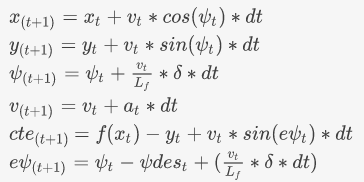
The update equations based on the previous parameters are:
These equations are used in the project to predict the state of the vehicle for the next 'N' timesteps.(lines 123-132 in mpc.cpp)
N- The number of timesteps in the horizon. dt - The time elapse between actuations The Product of N and dt is the prediction Horizon T- the duration for which the future predictions are made. As per Udacity guideline, T should be more and dt should be less.
int N = 10;
double dt = 0.1;
I used the value of N = 10 and dt = 0.1 suggested by some members in the forum. This gives a lookahead of one second.I tried to increase N to 20 and reduce dt to 0.05 to get the same lookahead time. The car was driving erratically. I tried many combinations. Any other values for N and dt , the car wouldn't drive properly.
The feedback from the simulator are (main.cpp lines 90-95)
- Waypoints (ptsx,ptsy)
- Car Position (x,y)
- Car Orientation (psi)
- Speed (v)
The way points ,car position and car orientation are transformed from map coordinates to vehicles co-ordinates as it is convenient to use in the prediction equations.(lines 97-114 in main.cpp).Car position & orientation in vehicle co-ordinate is [0,0,0].
A polynomial fit is found from the way points(lines 129-141 in main.cpp) and cte and epsi is calculated from which the state of the car is obtained. A reference waypoint is generated with a distance spacing of 2.5 (lines 195-199 in main.cpp)
The actual waypoints are predicted based on the model.(line 155 in main.cpp)
auto vars = mpc.Solve(state,coeffs);
IPOPT solver is used to solve optimization problem here as MPC is posed as a optimization problem,wherein the polynomial/Waypoint is the cost/Objective function;the vehicle state and the control variable become the Design Variable for the solver and impose constraints with the Vehicle model so that the dynamics of the system are satisfied .
Latency is introduced to as to take in account of the delay in the time the control is sent to the vehicle and the values are actuated in the hardware. The lag compensation is achieved by applying the latency to the dynamic model when propagating the state. A constant latency of 0.1 (100 millisecs) is used. (mpc.cpp- lines 182-188).
 double latency = 0.1;//100 milliseconds
 x = x + v*cos(psi)*latency;
 y = y + v*sin(psi)*latency;
 psi = psi + v*delta/Lf *latency;
 v = v + a*latency;
 cte = cte + (v * sin(epsi) * latency);
 epsi = epsi + v * delta / Lf * latency;
Together with this, the MPC requires some tuning . After all MPC is just another controller and all the controllers requires tuning for smoother functioning. I had to penalise the cost of different errors (mpc.cpp lines 55-73)so that the car doesn't oscillate, and takes turns smoothly.
