Main	Development

CAD_to_OpenMC

This is a python package intended to establish an open source link between CAD tools in general and the nuetron and photon transport code OpenMC. It is inspired by Paramak, and borrows concepts from step_to_h5m.

Although most CAD-tools use some other internal and/or native representation for geometry, most, if not all, will be able to export to the STEP-file format. Therefore this is the format we use

CAD_to_OpenMC uses cadQuery and its links to OCCT

The code structure relies on a main class Assembly, which maintains the geometry in terms of a list of instances of the subclass Entity. A geometry is imported from a (set of) .step files into the entity-list. This list is passed on to a mesher-class which generates a meshed geometry.

Other options

CAD_to_OpenMC is certainly not the only package that tries to solve this problem. Other options include:

These two packages solve the same problem as CAD_to_OpenMC, and in fact in many cases are interchangeable. See for instance [benchmark-zoo] ( https://github.com/fusion-energy/model_benchmark_zoo ).

To install/set up in a virtual python environment

replace <name> with an arbitrary name for your virtual environment

In the directory where you want your environment to reside do: python -m venv <name>
Activate the environment: source <name>/bin/activate
Build and install moab (if not already installed). The moab team relies on conda for standard installation but are working on a pip-based solution. Once that is done moab would simply be added to the requirements-file instead.
1. Clone the moab code-repository: e.g. git clone git@bitbucket.org:fathomteam/moab.git
2. Configure and build the code:
```
  mkdir build;
  cd build; cmake .. -DENABLE_PYMOAB=1 -DENABLE_HDF5=1 -DCMAKE_INSTALL_PREFIX=<name>;
  make;
  make install;
```
1. Additionally you will need to build the python interface layer.
```
  cd pymoab
  sudo python setup.py install
```
Install the main package: pip install CAD_to_OpenMC. This will pip-install all the required python packages in the virtual environment. This ensures that no additional conflicts are introduced with the system python.

Should you wish to install the development version of this package you may do so by cloning this repository and replace the last command by: pip install <path/to/repo>. This procedure will build and install the python package locally directly from source.

Optionally install the msh refinement tool mmg (https://www.mmgtools.org), which may be run in conjunction with the cq/stl-mesher backend to avoid the high aspect ratio triangles that this backend tends to produce. Arch-linux users may install this from the AUR, otherwise get the source (and build from that) or binary builds from the mmg-site.

To install in a conda environment

replace <name> with an arbitrary name for your virtual environment

If instead you prefer to use a conda-environment, this is now as simple as:

create an environment, e.g. conda create -n <name>
activate it: conda activate <name>
install CAD_to_OpenMC: conda install cad-to-openmc

Known problems

At present the parallel meshing option is buggy - it is therefore highly recommended to set the mesher to only use 1 thread. The team is working on a solution for this. See issue #80
Geometries which lead to degenerate toroidal surfaces in the step-files, can have problems. See issue #94
As is reported in #98 on Ubuntu 22.04 there's a problem with python 3.12. Specifically with installing "nlopt", which is used by one of the dependencies of CAD_to_OpenMC. We recommend to stay with python < 3.11 until this has been fixed upstream.

Use cases

We will show a few very simple uses-cases below to get you started using CAD_to_OpenMC, starting with a simply utility script, and then some more examples showing a few of the options later.

Simple utility script

This is the fastest way of getting up and running. A very basic script to process the file 'geometry.step' into a geometry useful for OpenMC in the 'geometry.h5m':

import CAD_to_OpenMC.assembly as ab

A=ab.Assembly('geometry.step')
ab.mesher_config['threads']=1
ab.mesher_config['tolerance']=1e-2
ab.mesher_config['angular_tolerance']=1e-2
A.run(h5m_filename='geometry.h5m',backend='stl2')

This may then be included in an openmc-geometry by this snippet e.g.:

import openmc
universe=openmc.DAGMCUniverse('geometry.h5m').bounded_universe(padding_distance=10)
geometry=openmc.Geometry(universe)

Please note that you also have to define materials according to the tags in the h5m-file for openmc to run.

7 pin test case

The follwing code-snippet can now be run to explore the capabilities of Assembly/step_to_h5m. We supply a couple of example .step-files in the examples directory. In this example we'll be using a geometry with a set of 7 pin-cells.

  import CAD_to_OpenMC.assembly as ab
  a=ab.Assembly()
  a.stp_files=["examples/7pin.step"]
  a.import_stp_files()
  a.solids_to_h5m()

as of version 0.2.6 a simpler version of this test-script may be used as we have added a small set of convenience functions. One possibility is:

  import CAD_to_OpenMC.assembly as ab
  a=ab.Assembly(['examples/7pin.step'])
  a.run()

which will read the 7pin.step example file and output a file by the default name dagmc.h5m

as usual.

Unless anything else is specified this procedure simply uses the default CAD_to_OpenMC parameters to create meshes using the default choice of meshing backend - namely gmsh. E.g. for the "gmsh"-backend this means sampling curves 20 times, a minimum mesh-element size of 0.1, and a maximum mesh element size of 10. This procedure will in turn call OCP and gmsh to produce a mesh with merged surfaces in the output file "dagmc.h5m"

The other available meshing backends are based on stl-export from CadQuery (accessible by setting backend='stl', or backend='stl2') which uses the parameters tolerance and angular_tolerance to set meshing quality. E.g. choosing the 'stl2' backend would alter the call to run to:

  a.run(backend='stl2')

Similarly the output filename may be set using the parameter h5m_filename.

Meshing parameters are changed by means of altering entries in the mesher_config-dictionary defined in the assembly module root namespace. Like:

 ab.mesher_config['min_mesh_size']=0.2

Below is a list of the available parameters and their meanings:

min_mesh_size

Minimum mesh element size (gmsh backend/mmg_refinement)

max_mesh_size

Maximum mesh element size (gmsh backend/mmg_refinement)

curve_samples

The number of point samples used to approximate a curve, 1D-mesh. (gmsh backend)

mesh_algorithm

Integer specifying which meshing algorithm to use (gmsh backend) 1: Adaptive algorithm - most often the most robust choice.

vetoed

A list of surfaces that should be excluded from meshing. Useful when some surface fails for whatever reason. Be aware that this may make your geometry non-watertight.

threads

The number of threads to be used to speed up the meshing algorithms. Useful for multicore-computers.

tolerance

angular_tolerance

Relative angular mesh tolerance (stl/stl2 backends) Lower this to get a better angular resolution.

refine

After the initial meshing step is done, should the mesh be refined?

This option has more than one meaning depending on which backend you have chosen.

If the cq/stl-backend is active and the refine option is non-zero or True, the mesh-refinment tool (mmg)[https://www.mmgtools.org] is called in sequence on each surface.
If the gmsh-backend is active and the refine option is non-zero the gmsh-refinement tool is called on the full geometry the given number of times. A value of True is the same as setting the option to 1, i.e. it triggers a single loop through the refinement algorithm.

verbose

Output lots of information from the mesher backends.

As of version 0.3 We also distribute a utility script (in the scripts directory) that should be helpful in creating meshes. An example run could look like this, which furthermore sets the implicit complement to be air. (See below for more on implicit complement):

  c2omc_step2h5m examples/7pin.step --threads=1 --verbose=2 --implc=air --backend=stl2

For a description of all available command line options simply run

  c2omc_step2h5m --help

One noteable difference is that the default meshing backend is in this case 'stl2'

meshing backends

At present three different backends exist for CAD_to_OpenMC: 'gmsh', 'stl', 'stl2'. It is possible to add another backend should another meshing library become available.

gmsh

The inner workings of this backend is basically a simple call to gmsh to create a 2D-mesh of the entire geometry. This has the advantage that inhenrently boundary curves are meshed only once, meaning that in theory, they can be made to account for shared surfaces without unwanted artefacts. At its present stage however there may be problems with leakage when performing transport calculation on geometries with shared surfaces. A significant drawback todoing the entire geometry all at once, is that for larger geometries memory requirements may be prohibitive.

stl

The stl backend takes a different approach. Instead each solid object in a step geometry is triangulated on its own. The triangulation itself is performed by calls to the underlying OpenCASCADE-library through the python layer cadquery. This procedure sidesteps the problem with large geometries, as each object in handled on its own. Objects cannot overlap however, and just as the case is for the gmsh-backend, surfaces should not be coincident.

stl2

As its name implies the stl2 backend builds on concepts from the stl backend. However a major difference lies in the fact that objects can now have coincident surfaces. This is achieved by splitting the tringulation operation further and instead perform it in a face-by-face manner. This way we may skip the operation is one face (or surface) is a part of two solids. Furthermore, when the surfaces are assembled into a h5m datafile, the surfaces may be appropriately flagged such that transport algorithms can handle moving from one to another. If this is important for your problem, then this is the backend you should use.

implicit complement

CAD_to_OpenMC supports the notion of an implicit complement material, i.e. a material that fills all the space within the geometry which has not been claimed by any part in the CAD-assembly. For instance if one wanted to submerge a pincell in in water it is possible to only define the pincell as part and set the implicit complement material to water. To do so we would use code like:

import CAD_to_OpenMC.assembly as ab
a=ab.Assembly()
a.implicit_complement='water'
...

Of course, this means that the subsequent OpenMC transport simulation needs to define a material (with the wanted properties) named 'water'.

Intermediate datafiles

In the process of generating an .h5m-geometry file CAD_to_OpenMC also generates a sometimes large amount of intermediary datafiles, these may be retained for debugging purposes (the default), but by setting a flag, CAD_to_OpenMC can be directed to delete them automatically once they're no longer needed. Since version 0.3 the intermediate datafiles are put in a newly created subdirectory, named <h5m_file_stem>_DATE_TIME. The cleanup-flag is set as such:

import CAD_to_OpenMC.assembly as ab
a=ab.Assembly()
a.cleanup=True

Merging a set of geometries

If you have non-overlapping geometries, it can be convenient to mesh them separately, e.g. to save memory, only to merge them at a later stage. In CAD_to_OpenMC this is supported (since 0.3.1) through a utility function merge2h5m. Imagine you have two step-files: one.step and two.step which you know to not overlap, but you would like them to belong to the same geometry/scene. In this case you may create a single h5m-file containing them both by means of the follwing procedure.

import CAD_to_OpenMC.assembly as ab
One = ab.Assembly(['one.step])
One.run(backend='stl2', merge=True, h5m_filename='one.h5m')

Two = ab.Assembly(['two.step])
Two.run(backend='stl2', merge=True, h5m_filename='two.h5m')

ab.merge2h5m([One,Two],h5m_file='three.h5')

This will run the normal triangulization procedure for one and two separately, but also create a single h5m-file: three.h5m which contains both of the geometries.

Advanced example

For a more advanced example of the use of CAD_to_OpenMC and OpenMC we may turn to the Zero Power Reactor Experiment. This was a full-scale reactor experiment that was carried out at Oak Rodge TN in the 1960's. Copenhagen Atomics provides a CAD-drawn model of this experiment, extracted from the original reports and drawings from the original experiment, in the form of a step-file. To get access simply clone the zpre github repository and run the scripts:

git clone https://www.github.com/openmsr/zpre
cd zpre
bash run.sh

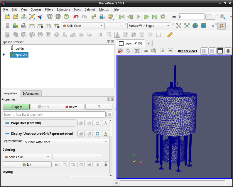
The run.sh-script will the ask you what kind of calculation you'd like to perform. As a first run you might choose to ask OpenMC to simply plot the geometry of the reactor (option 2). If this is the first time you run the script, this triggers a surface-meshing operation to be performed (Be aware that by default this creates a large amount of console output - this is to be expected). During the surface meshing operation (by default) a .vtk-file is created in addition to the .h5m-file that OpenMC (and DAGMC) needs. This is for convenience so you may inspect the created mesh using e.g. paraview, if you have access to that. If you have paraview installed the call paraview h5m_files/zpre.vtk should yield a geometry like this .

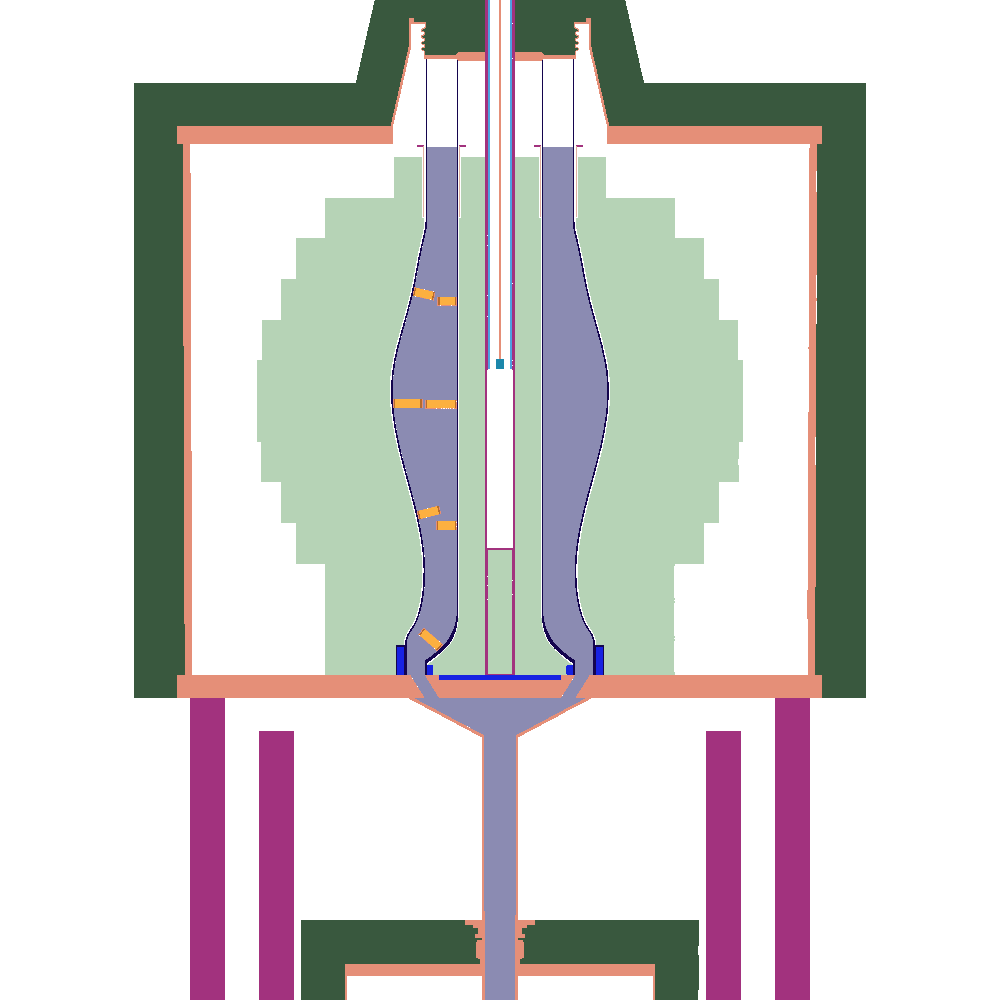
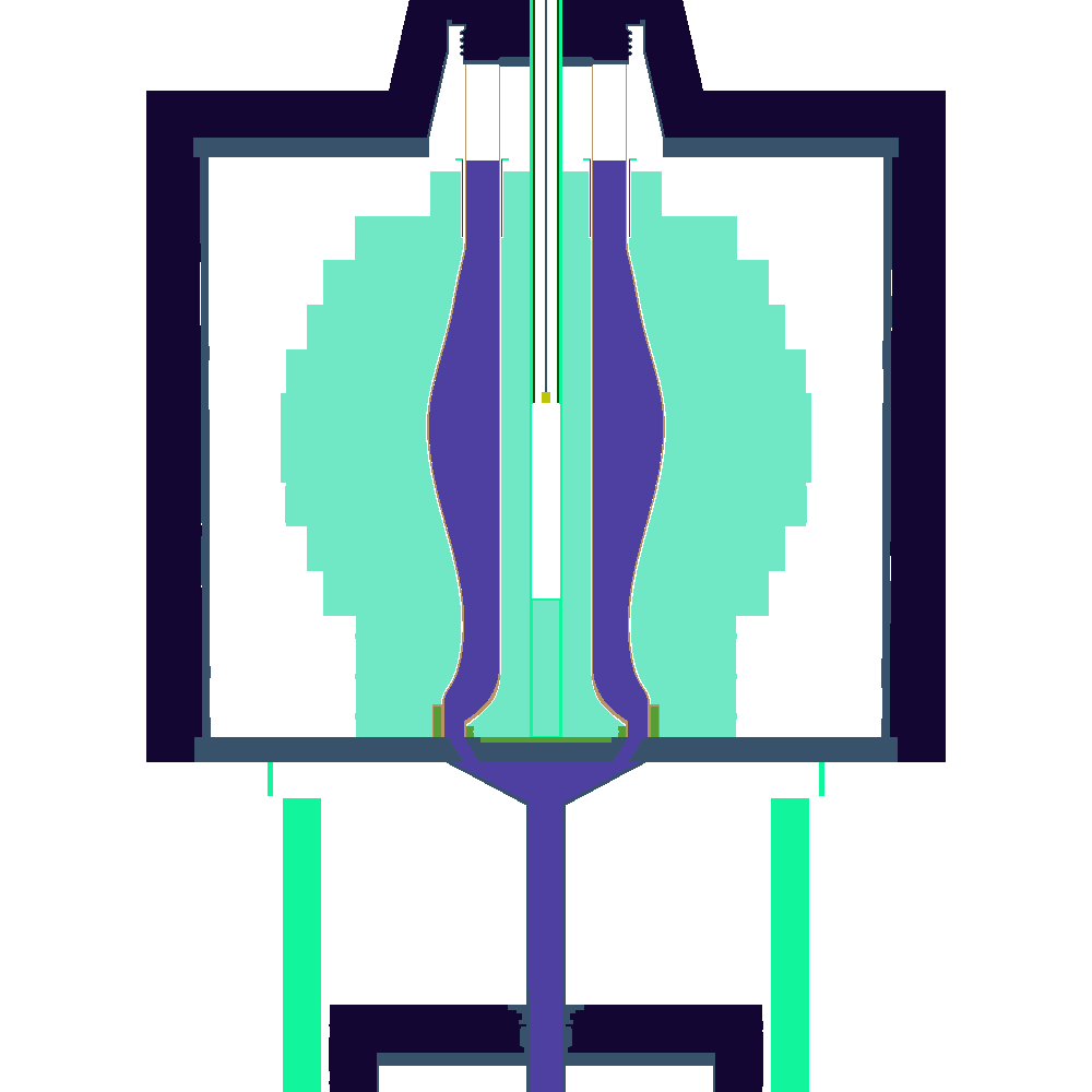
Once this process has finished, there should now be a file zpre.h5m inside the h5m_files directory, and a set of plot_[123].png files. which correspond to XY,XZ, and YZ-slices through the center of the reactor. If all goes well these should look something like this:

XY	XZ	XZ

The colors are chosen arbitrarily amd automatically by the OpenMC-plotting routine, which is why the same geomtrical entity gets a different color in the slices.

moatazharb/CAD_to_OpenMC