value-rnn-td: A Python repository from mobeets

Installation

conda create --name valuernn python=3.9 pytorch matplotlib numpy scipy scikit-learn
conda activate valuernn

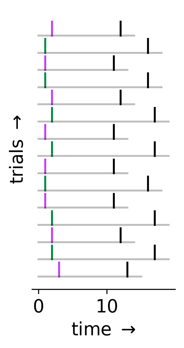
Training an RNN to learn value using TD learning

Example experiment

In the provided example experiment, each trial consists of a cue, X (either magenta or green), followed by a reward, r (black), that arrives a fixed number of time steps later (magenta = 10, green = 15). In other words, for a trial where X(t) = green, we will have r(t + 15) = 1.

Training an RNN to do TD learning

We can define the "value" of being at time t as the expected cumulative reward, V(t) = E[r(t) + γr(t+1) + γ^2r(t+2) + ... ], where future rewards are discounted by a factor 0 ≤ γ ≤ 1. We would like to train a network to estimate value at each time step given only our history of observations, X(1), X(2), ..., X(t), r(1), ..., r(t-1).

To estimate value, we will train an LSTM with two hidden units using TD learning. Specifically:

At each time step, our network's output will be Vhat(t) = max(0, z1(t)) + max(0, z2(t)), where z1(t) and z2(t) is the activity of our two hidden units.
In TD learning, we estimate all future rewards as γVhat(t+1) ("bootstrapping"), so our goal is to get Vhat(t) as close to r(t) + γVhat(t+1) as possible. In other words, the network's error at each time step is δ(t) = r(t) + γVhat(t+1) - Vhat(t), where δ(t) is called the "reward prediction error."
To update our network's parameters, θ, we use stochastic gradient descent: Δθ = αδ(t)g(t), where α is our step size, and g(t) is the gradient of Vhat(t) with respect to θ. (TD learning in this case is equivalent to minimizing the mean squared error between our target, r(t) + γVhat(t+1), and our prediction, Vhat(t).)

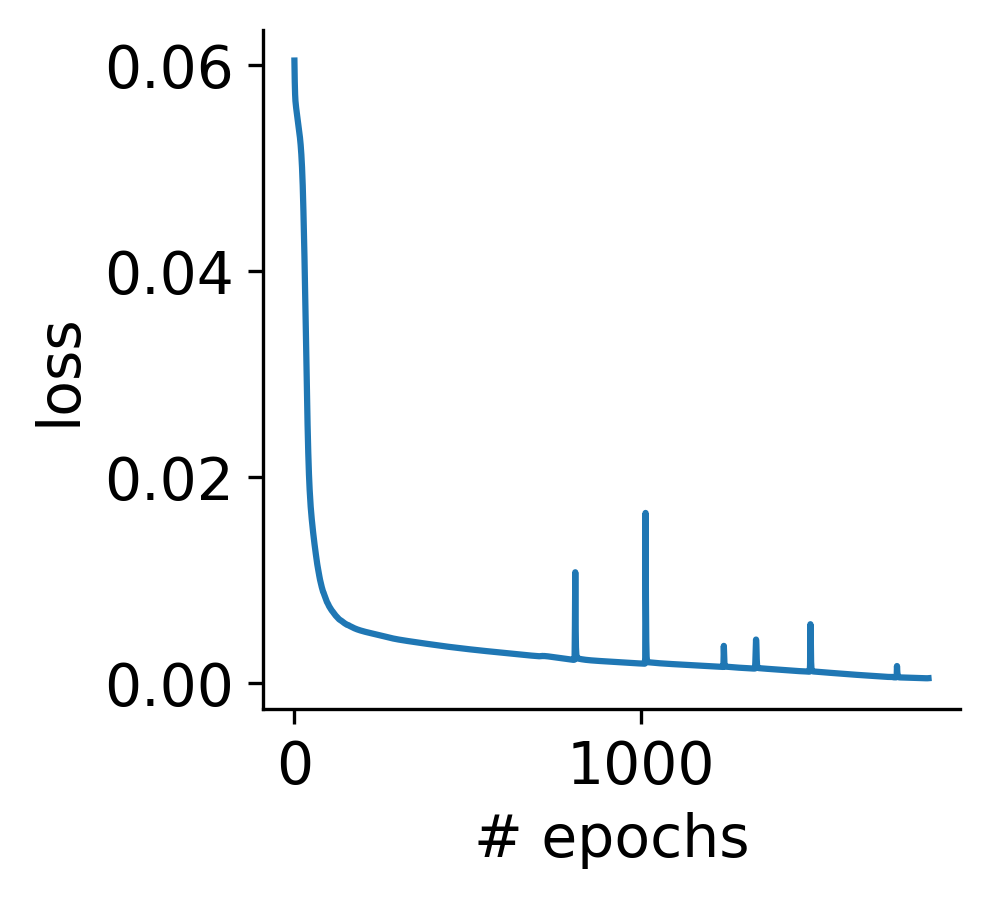
For this example, we'll set γ=0.5. Below, we train our network using stochastic gradient descent (with backpropagation through time) with the Adam optimizer. Training is complete after roughly 2000 epochs.

Inspecting the RNN

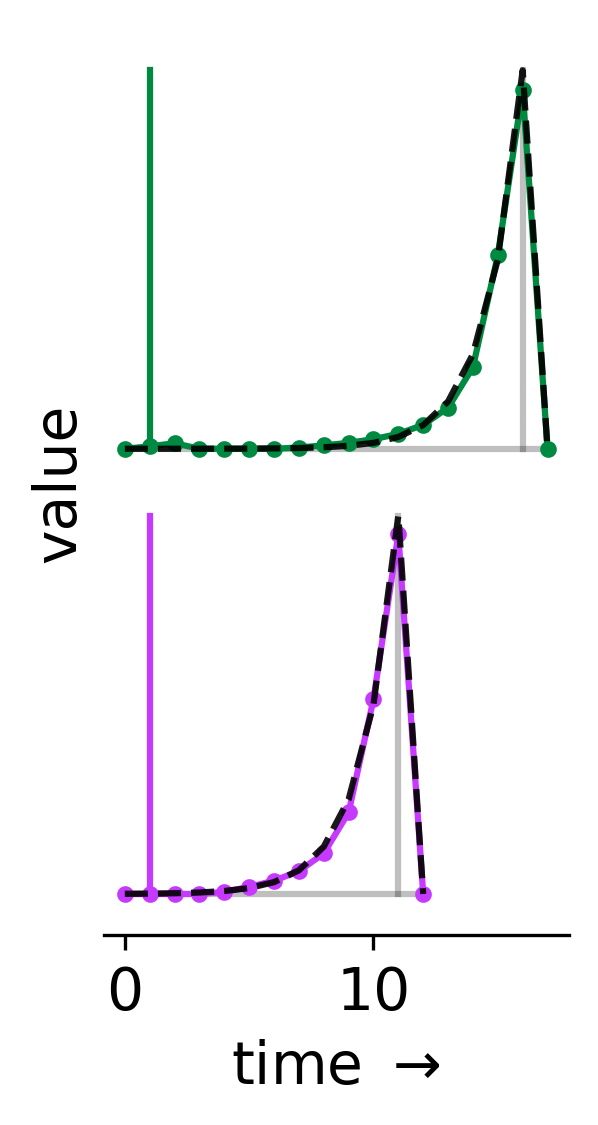
Because this is such a simple task, we actually know the true value function. Specifically, we have V(t) = γ^(c - t) for 0 ≤ t ≤ c, where c = 10 for trials with a magenta cue, and c = 15 for trials with a green cue. We can see how well our network has learned these two value functions. Below, the colored lines depict Vhat(t) on the two types of trials, and the black dashed lines indicate the true value, V(t).

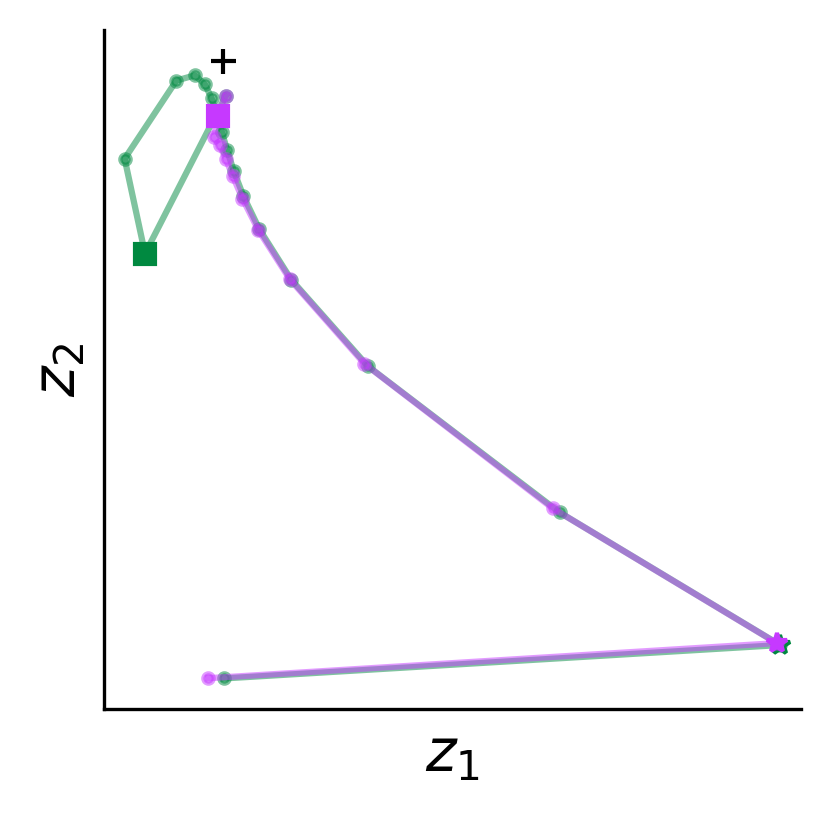
Remember that Vhat(t) is the summed output of the LSTM's two hidden units, z1(t) and z2(t). Below, we can visualize how this activity evolves during these two example trials. The squares indicate the time step on each trial when the cue was presented, while the stars indicate when reward was delivered. Note that these are the only two times in each trial when the network's input is non-zero.

Features

Though the above example is very simple, training such a network using pytorch involves a few tricky steps. This includes: