Python Sphere RCS Calculator

This library uses the Mie Series to compute the Radar Cross Section for a lossy dielectric sphere. The Radar Cross Section (RCS) can be plotted for a variety of test scenarios, such as:

mono-static RCS versus frequency for one or many spheres
bi-static RCS for one or many spheres with different materials
bi-static RCS for one sphere at multiple frequencies

The code is supplemented by several functions for generating, saving, and plotting RCS data. Since the Mie Series produces an analytical result, this code can be used to verify results obtained using numerical computational electromagnetic solvers.

This code is primarily based on the following works:

C. A. Balanis, Advanced Engineering Electromagnetics. New York, NY: John Wiley & Sons, Inc., 1989.
G. Kevin Zhu (2021). Sphere scattering (https://www.mathworks.com/matlabcentral/fileexchange/31119-sphere-scattering), MATLAB Central File Exchange.
W. J. Wiscombe, "Improved Mie scattering algorithms," Appl. Opt. 19, 1505-1509 (1980)
Allardice, J. R., & Le Ru, E. C. (2014). Convergence of Mie theory series: criteria for far-field and near-field properties. Applied Optics, 53(31), 7224. doi:10.1364/ao.53.007224

Contributors to this library:

Iliya Shofman, Damian Marek, Shaswat Sharma, Piero Triverio

Overview of Library

Code Requirements

Python version 3.x
numpy, matplotlib, scipy.special, mpmath

Coordinate System

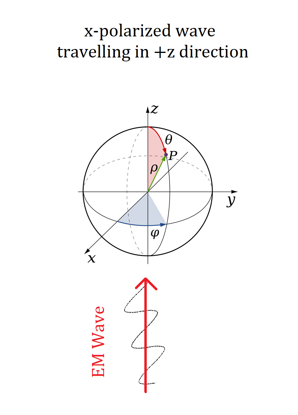
The calculations in this library assume that an x-polarized wave travels in the positive z- direction. Theta (the polar angle) is zero at the positive z-axis, reaches maximum value of pi at the negative z-axis. Phi (the angle of azimuth) is zero at the positive x-axis.

To observe differences caused by plane wave polarization in the bistatic case, change the phi variable. For example, to see RCS from y-polarized waves, set phi = pi/2. For circularly polarized waves, compute as a linear superposition of two modes.

List of Function Arguments

This library makes use of the following parameters when computing the Radar Cross Section of dielectric spheres:

radius (meters) - the radius of the sphere
ratio (unitless) - ratio of sphere radius to wavelength
frequency (Hertz) - the frequency of impinging plane wave
sensor location - an (x,y,z) coordinate in meters at which the RCS is evaluated. The sphere is positioned at the origin.
sphere_material and background_material - objects of class DielectricMaterial
save_file (string) - output file names for saving data

Class Definitions

This library makes use of several classes to organize the process of passing arguments to functions:

DielectricMaterial: defines a medium by its electric permittivity, electric conductivity, and magnetic permeability as DielectricMaterial(eps_r, sigma_e=0, mu_r=1, sigma_m=0, name=None). For example, a silicon nanoparticle with a conductivity of 10 S/cm can be defined as doped_silicon = DielectricMaterial(11.7, 10, 1). Note: a Perfect Electric Conductor can be defined by setting electric permettivity to a large value and magnetic permeability to a small value such that their product equals 1, for example, PEC = DielectricMaterial(1e8,0,1e-8,0) (See Balanis referene).

For comparing the RCS between multiple spheres or positions, the use of the TestCase and TestParameters classes are encouraged.

TestCase - defines a sphere of some radius and material immersed in a specified medium as, for example, PEC_nanoparticle_in_silicon = TestCase(radius = 1e-7, sphere_material = PEC, background_material = doped_silicon)
TestParameters - groups together the sensor location and frequencies at which the RCS is to be tested for. Following the earlier example, we could call test_1 = TestParameters([0,0,-1e-5], 2.4e9).

List of Functions

Using these parameters, the following functions are defined for this library:

(Monostatic RCS)

RCS_vs_freq (radius, ratio, background_material, sphere_material, sensor_location, save_file)
plotOneMonoRCS (radius, sphere_material, background, mono_RCS, ratio, savefile)
saveMonoRCSData (savefile, mono_RCS, frequency, sphere, radius)
Compare_RCS_vs_freq (test_cases, test_parameters, save_file)

(Bistatic RCS)

Bistatic_RCS (radius, frequency, background, sphere, distance, phi)
plotBiRCS (radius, sphere, frequency, bi_RCS, theta, savefile)
saveBiRCSData (savefile, bi_RCS, theta, frequency, sphere)
Compare_Bistatic_RCS (test_cases, test_parameters, save_file)

Example Usage

This section will show example code for creating frequently-used plots. This code can be pasted into the main function in the file getRCS.py. For questions about individual functions, please see the docstrings.

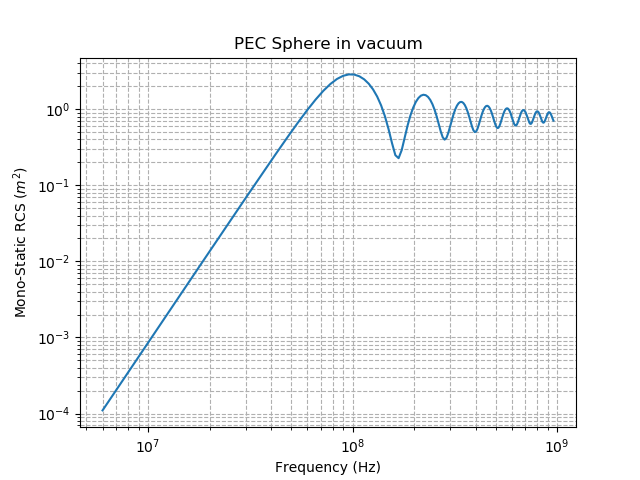
Mono-Static RCS vs Frequency for One Sphere

This example computes the monostatic RCS for a Perfect Electric Conductor. The material definition for the PEC comes from Balanis 1989. The code produces a plot (PEC.png) and saves the data to a text file (PEC.txt).

RCS_vs_freq(radius = 0.5, ratio = np.arange(0.01,1.61,0.01), \
            background_material = DielectricMaterial(1,0), \
            sphere_material = DielectricMaterial(1e8,0,1e-8,0), \
            sensor_location = [0,0,-2000], save_file = 'PEC')

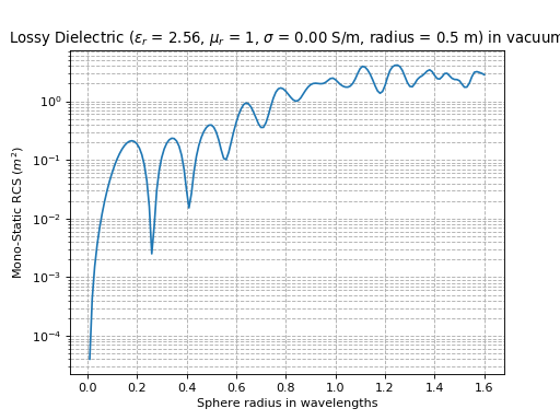
Note: the variable ratio is defined as radius / wavelength. To have the x-axis be in terms of ratio, use function plotOneMonoRCS(). This function accepts either ratio, frequency, or wavelength, and plots it on the x axis. :

radius = 0.5 #meters
ratio = np.arange(0.01,1.61,0.01)
background = DielectricMaterial(1,0)
sphere_material = DielectricMaterial(2.56,0.003)
sensor_location = [0,0,-2000] #meters

(freq, mono_RCS) = RCS_vs_freq(radius, ratio, background, sphere_material, \
                        sensor_location , save_file = 'PEC', show_plot = 0)
plotOneMonoRCS(radius, sphere_material, background, mono_RCS, ratio = ratio, \
                savefile = "lossy_dielectric_mono_rcs")

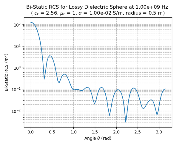
Bi-Static RCS (vs angle) for One Sphere

The code sample below displays a plot of Bistatic RCS for a lossy dielectric sphere, and saves this data to a text file. The first function calculates and returns a numpy array with Bistatic RCS data, along with displaying the plot. The second function saves the data to a file, without saving the plot. To not display the plot, set show_plot=0.

radius = 0.5
background = DielectricMaterial(1,0)
sphere = DielectricMaterial(2.56,0.01)
distance = 2000 
phi = 0
(theta, bi_RCS) = Bistatic_RCS(radius, 1e9, background, sphere, distance, phi, show_plot=1)
saveBiRCSData("bistatic_perfect_dielectric_example", bi_RCS, theta, 1e9, sphere)

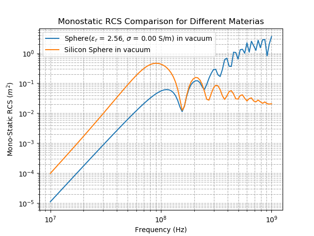
Mono-Static RCS vs Frequency for Multiple Spheres

For plotting multiple spheres, use the Compare_RCS_vs_freq() function, or the plotFromFile function. Each plot line represents RCS data for one TestCase, in which a sphere of size radius and material sphere_material is immersed in a background_material. Each TestCase can be evaluated under one or many TestParameters, which include sensor_location and frequency.

#class TestCase(radius, sphere_material, background_material)
case1 = TestCase(0.5, DielectricMaterial(2.56,0), DielectricMaterial(1,0))
case2 = TestCase(0.5, DielectricMaterial(2.56,0.1, name = "Silicon"), DielectricMaterial(1,0))

#class TestParameters(cartesian_sensor_location, frequency)
param1 = TestParameters([0,0,-2000], np.logspace(7,9,100))

Compare_RCS_vs_freq([case1,case2], param1, "example_2_material_comparison")

Conductivity Sweep

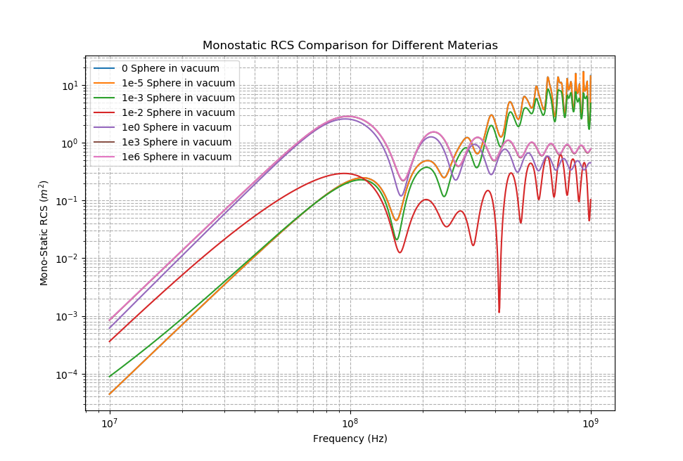
To plot the RCS of a sphere at many different conductivities, one can automate the process of creating TestCase objects like this:

vacuum = DielectricMaterial(1,0)
radius = 0.5
conductivities = [0, 1e-5, 1e-3, 1e-2, 1e0, 1e3, 1e6]
names  = ["0", "1e-5", "1e-3", "1e-2", "1e0", "1e3", "1e6"]
eps_r, mu_r = 2.56, 1

cases = []
for i in range(0, len(conductivities)):
    sphere = DielectricMaterial(eps_r, conductivities[i], mu_r, name = names[i])
    test_case = TestCase(radius, sphere, vacuum)
    cases.append(test_case)

sensor_location = [0,0,-2000]       #[x,y,z], all in meters
frequency = np.logspace(7,9,1000)
param1 = TestParameters(sensor_location, frequency)

Compare_RCS_vs_freq(cases, param1, save_file = "sigma_sweep_kzhu_nmax")

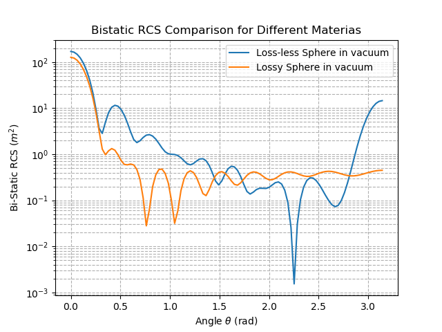
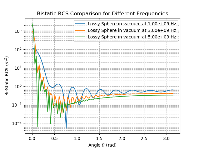
Bi-Static RCS for one Sphere at Multiple Frequencies

Using the function Compare_Bistatic_RCS, one can compare the RCS of multiple spheres at the same frequency, or one sphere at multiple frequencies. This example shows both.

Bistatic RCS for two spheres, one frequency

vacuum = DielectricMaterial(1,0)
radius = 0.5
sphere1 = DielectricMaterial(2.56,0, 1,0, name = "Loss-less")
sphere2 = DielectricMaterial(2.56,1, 1,0, name = "Lossy")
test_cases = [TestCase(radius, sphere1, vacuum), TestCase(radius, sphere2, vacuum)]

sensor_location = [0,0,-2000]
frequency = 1e9
test_parameters = TestParameters(sensor_location, frequency)

Compare_Bistatic_RCS(test_cases, test_parameters, save_file = "compare_bistatic_materials")

Bistatic RCS for one sphere, two frequencies

vacuum = DielectricMaterial(1,0)
radius = 0.5
sphere3 = DielectricMaterial(2.56,3.3, 1,0, name = "Lossy")
test_cases = [TestCase(radius, sphere3, vacuum)]

sensor_location = [0,0,-2000]
frequency = [1e9, 3e9, 5e9]
test_parameters = TestParameters(sensor_location, frequency)

Compare_Bistatic_RCS(test_cases, test_parameters, save_file = "compare_bistatic_frequencies")

modelics/Python-Sphere-RCS