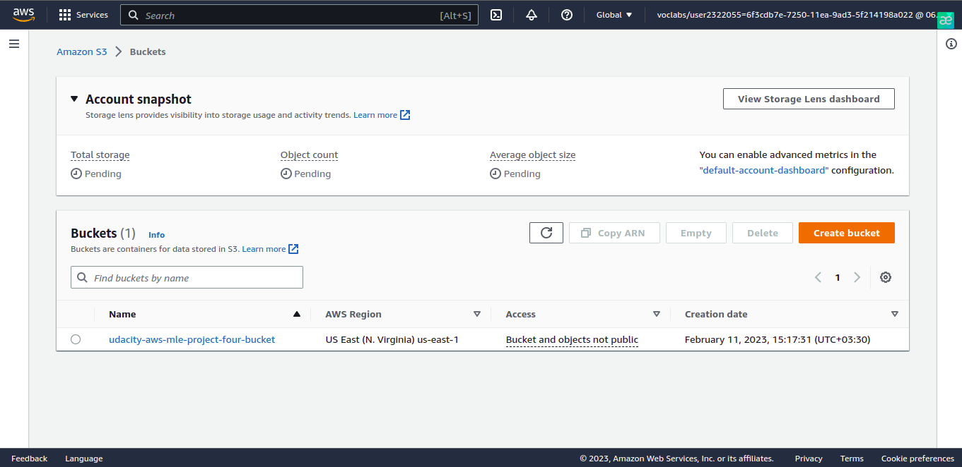
Operationalizing an AWS ML Project

In this project, we'll start with a completed ML project. Our goal in this project will be to use several important tools and features of AWS to adjust, improve, configure, and prepare the model we started with for production-grade deployment.

Note: This repository relates to AWS Machine Learning Engineer nanodegree provided by Udacity.

Taking raw ML code and preparing it for production deployment is a common task for ML engineers, and it's very important for the following reasons:

ML code alone isn't sufficient for most business scenarios. Real business situations require ML code to integrate with other infrastructures, like API's, applications, or other websites that require ML code to be correctly configured.
If ML code is deployed in a way that's not optimal, it can lead to cost overruns or bad performance.
When ML code is moved to production deployment, security is always a concern, since poor security can lead to data leaks or performance issues.

Project Summary

Train and deploy a model on Sagemaker, using the most appropriate instances. Set up multi-instance training in our Sagemaker notebook.
Adjust our Sagemaker notebooks to perform training and deployment on EC2.
Set up a Lambda function for your deployed model. Set up auto-scaling for our deployed endpoint as well as concurrency for our Lambda function.
Ensure that the security on our ML pipeline is set up properly.

Initial setup

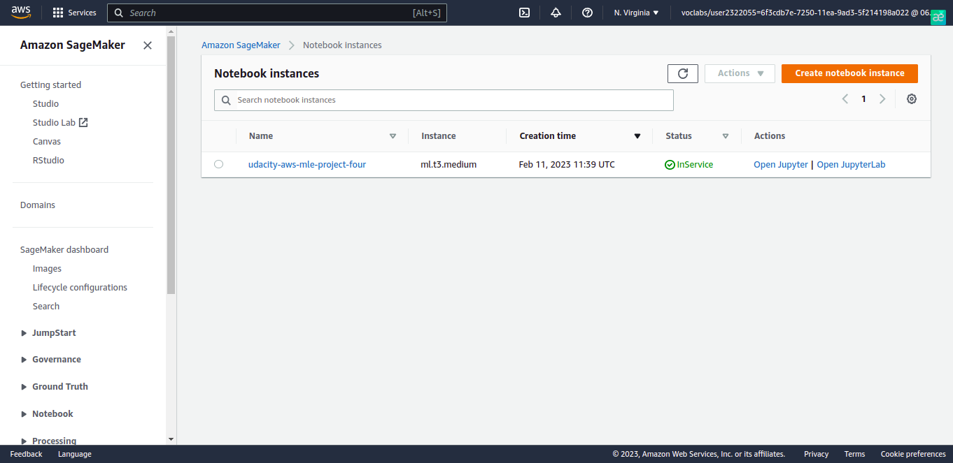
First, we create and open a Sagemaker instance from Notebooks > Instances section of AWS SageMaker. After creating the instance, it's running as shown below:

Due to this link, the ml.t3.medium is a suitable option to choose the notebook instance type: fast launch, CPU-intensive, and offering a balance of compute, memory, and network resources. For training, I chose the ml.m5.xlarge instance type due to its acceptable time processing and resource consumption.

Download data to an S3 bucket

The first three cells of the train_and_deploy-solution.ipynb will download data to our AWS workspace.

Training and Deployment

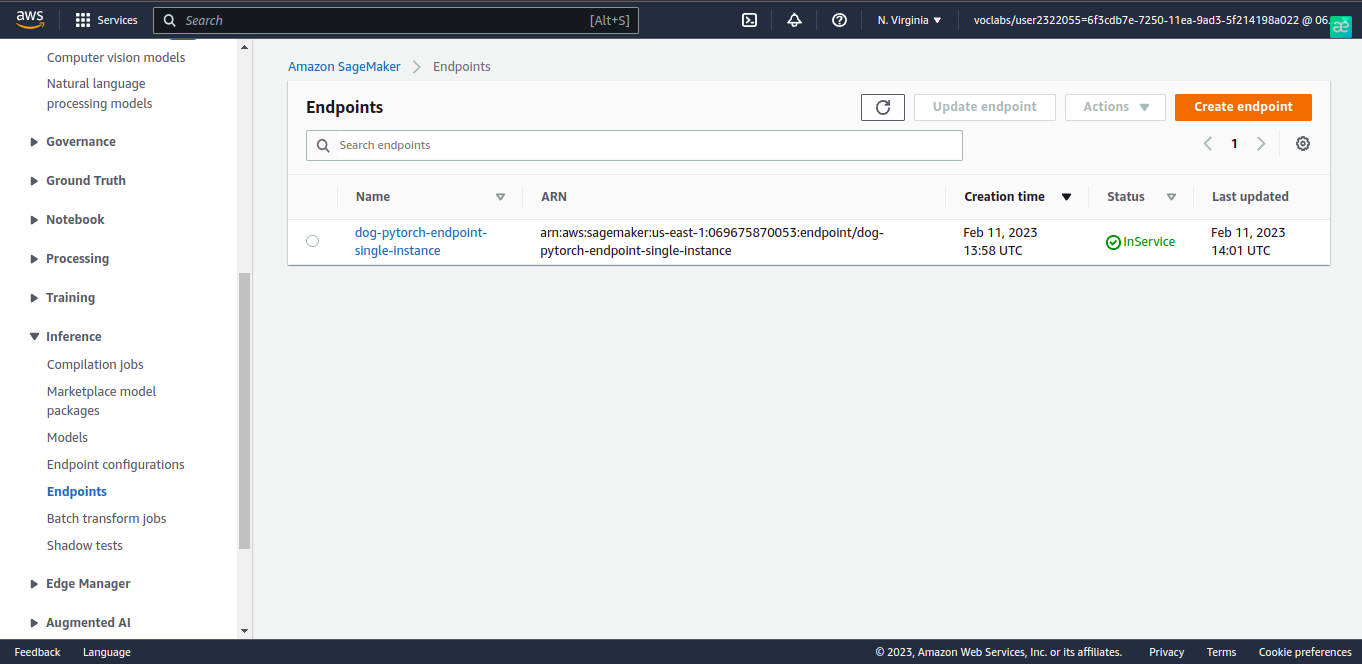
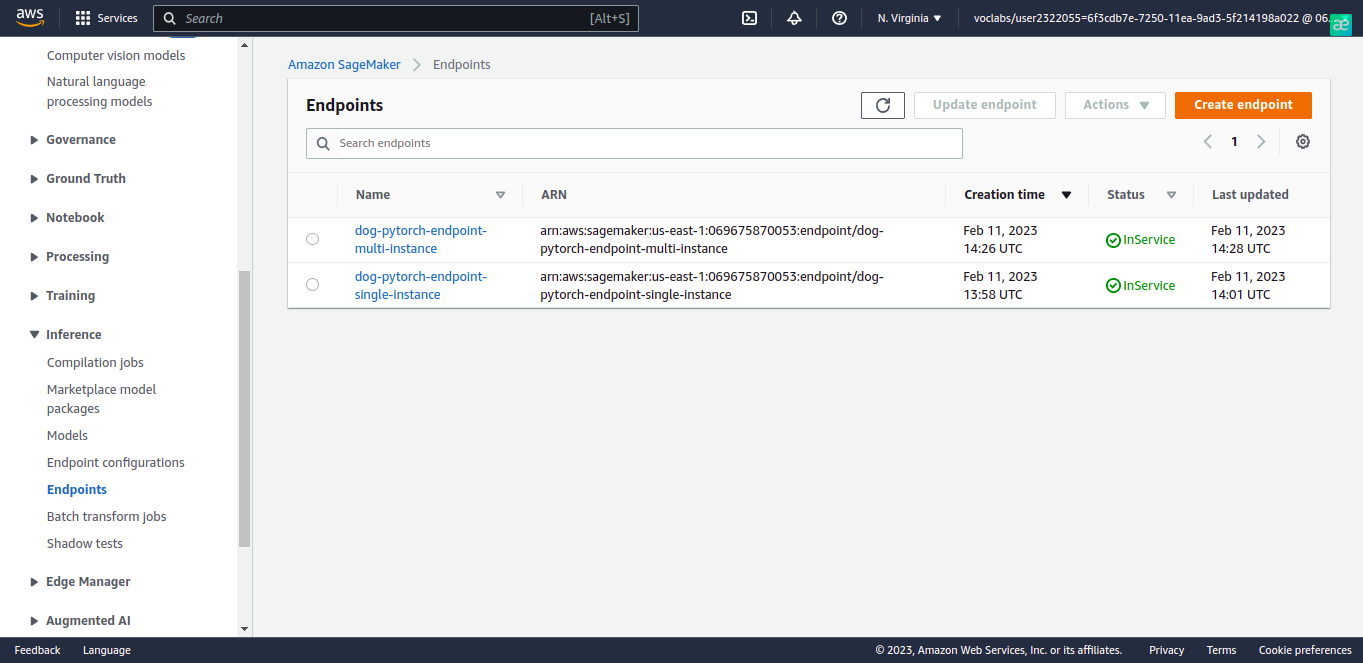
We run remaining cells in train_and_deploy-solution.ipynb. This finds the best hyperparameters for training our model, trains our base ResNet50 model in both single-instance and multi-instance trainings, and deploy an endpoint to Inference > Endpoints section of AWS SageMaker account.

For switching between single-instance and multi-instance training, it's just to change the value of instance_count parameter in sagemaker.pytorch.PyTorch class instantiation.

single-instance training endpoint

multi-instance training endpoint

EC2 Training

The next step is to set up an EC2 instance and accomplish model training there.

We create an EC2 instance and connect to it. We have a typical task which needs a balance of time, computation and networking resources. As described in here and here, then we can choose a general purpose instance. Among these instances, I chose ml.m5.xlarge instance type due to its acceptable time processing and resource consumption and shining former experience I had when I was working with.

After we've connected to the instance, obtain the data we need for training, by running the following two commands in our EC2 terminal:

wget https://s3-us-west-1.amazonaws.com/udacity-aind/dog-project/dogImages.zip
unzip dogImages.zip
mkdir TrainedModels
nano solution.py
# TODO: Paste all of the code from the starter file called ec2train1.py into this file. After that, save and close the 
# file.
python solution.py

As we can see in the screenshot below, the mode is trained and saved into TrainedModels directory.

Setting up a Lambda function

After training and deploying our model, setting up a Lambda function is an important next step. Lambda functions enable our model and its inferences to be accessed by API's and other programs, so it's a crucial part of production deployment.

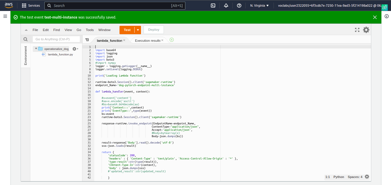
We need to set up a Lambda function that uses Python 3 for its runtime.lambdafunction.py contains the logic of the Lambda function with an endpoint corresponds to single-instance/multi-instance training.

You can test both single-instance and multi-instance training endpoints by change the endpoint_name variable in lambdafunction.py.

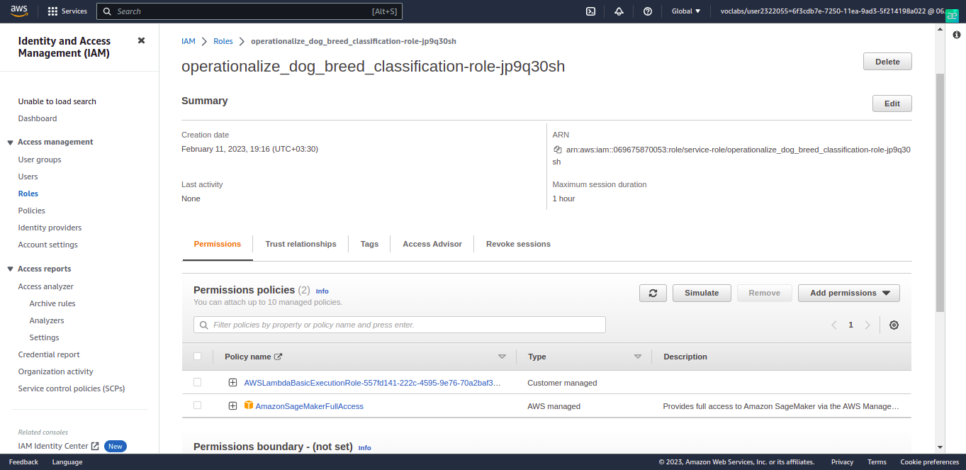
Then we'll have to find the "role" that the lambda function is using in the IAM interface, attach the correct security policy to the role of the lambda function. The security policy we attach should be one that allows our lambda function to access all of our SageMaker endpoints.

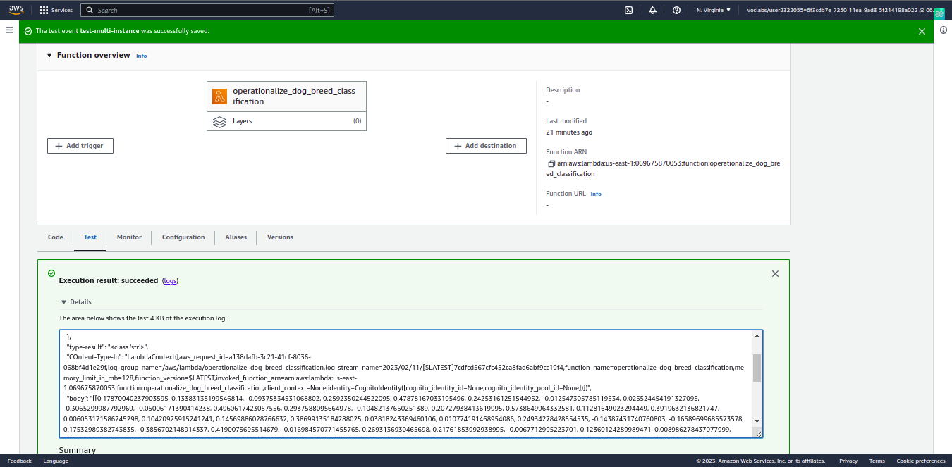
After resolving the lambda function security issue, we can test our lambda function. We can use the following text for our test event:

{ "url": "https://s3.amazonaws.com/cdn-origin-etr.akc.org/wp-content/uploads/2017/11/20113314/Carolina-Dog-standing-outdoors.jpg" }

We can see the result of the test event above:

Concurrency & Auto-scaling

We should set up concurrency for our Lambda function. Concurrency will make our Lambda function better able to accommodate high traffic because it will enable our function to respond to multiple invocations at once. We used provisioned concurrency since we have a requirement receiving a lot of traffic, so we need an automatic way for handling that. So we set provisioned concurrency to 3.

In addition to setting up concurrency for our Lambda function, we should also set up auto-scaling for our deployed endpoint. Due to the strength of the instance type we chose(ml.m5.xlarge), we set maximum_instance_count to 3. We also set the target value at the configuration of auto-scaling to 25 because we think it’s a suitable threshold to trigger the auto-scaling mechanism. If we choose a small number, then the auto-scaling is over triggered even if it’s not needed. If we choose a high number, then the auto-scaling may never be called. Scale-in and scale-out cool down values were both set to 30 seconds due to a balance of resource management, cost management and time acceptability.

mohsenMahmoodzadeh/operationalizing-an-aws-ml-pipeline