1. Description
2. Data Creation
3. Data Augmentation
4. Model
5. Evaluation
6. Setting up your machine
7. Setting up UI
8. Setting up Firebase
9. Setting up Backend
10. Flowchart
11. Usage
12. Dashboard
This project is about German Traffic Sign Recognition and uses the German Traffic Sign Recognition Benchmark Dataset to train the model. It has a user friendly Ui which provides the user a easy and interactive way to use this model. It is built with NextJs and Flask for the forntend and backend respectively. User will have the ability to add specific images using a level of randomization to the dataset, for every class. Users will also be provided with reasonable control over the type of augmentations, transformations to be added to the images. The user will be able to visualize the additional images after augmentations, transformations and will also have the freedom to balance the updated dataset, curate it and split it into train and validation. Moreover the UI will allow users to easily play with the metrics which will provide the reason and information if the network fails in some place or what steps should be taken to make the experiment work.
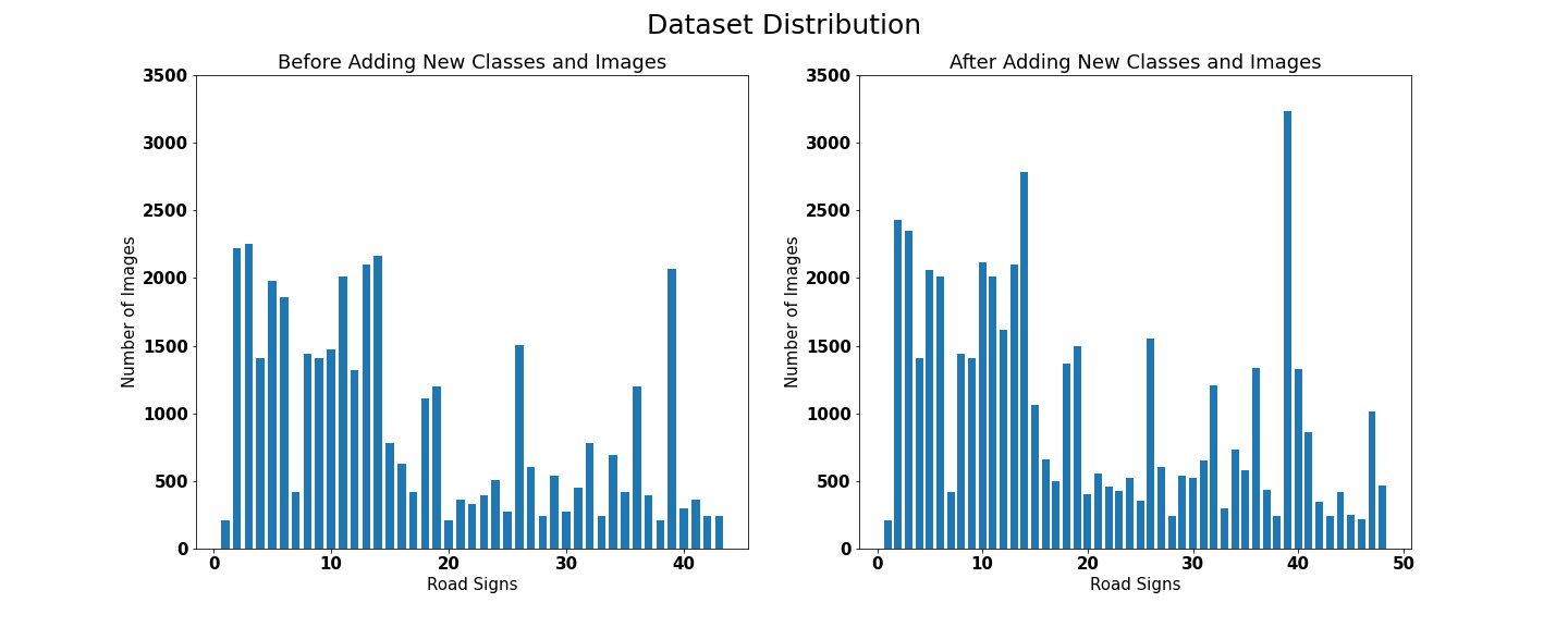
We use the GTSRB dataset (German Traffic Sign Recognition Benchmark) provided by the Institut für Neuroinformatik group. Images are spread across 43 different types of traffic signs and contain a total of 39,209 train examples. As per our analysis of the dataset, it is very unbalanced, some of the classes having 2000 samples, and some of them having only 200 samples. Although the images in each class of the dataset have some variance the number of images in some classes is so shallow that we had to append images to the existing dataset further to improve its variance. Although we couldn’t compensate for the class imbalance present in the dataset, our aim in adding the new images was to improve the overall diversity of the dataset
We introduced 5 new classes which consist of signs for the bus stop, crossing ahead, no stopping, no priority road, and school ahead to the dataset by scraping data from the internet. The dataset consists of images of only the road signs rather than a whole scene, so our proposed model could identify a road sign more effectively if the input of only the cropped road sign is fed to it rather than a whole scene which consists of the road sign.
We implemented the original IDSIA MCDNN model with an extra batch normalization layer and several other modifications.
We use the following regularization techniques to prevent overfitting:
Dropout : A simple way to prevent neural networks from overfitting. Dropout is a regularization method that approximates training a large number of neural networks with different architectures in parallel. During training, some number of layer outputs are randomly ignored.
Batch Normalization : During training time, the distribution of the activations is constantly changing. The intermediate layers must learn to adapt themselves to a new distribution in every training step, so training processes slow down. Batch normalization is a method to normalize the inputs of each layer, to fight the internal covariate shift problem.
Early Stopping : A major challenge in training neural networks is how long to train them. If we use too few epochs, we might underfit; if we use too many epochs, we might overfit. A compromise is to train on the training dataset but to stop training at the point when performance on a validation dataset starts to degrade. This simple, effective, and widely used approach to training neural networks is called early stopping. We used early stopping with a patience of 100 epochs. After the validation loss has not improved after 15 epochs, training is stopped.
The problem with CNN’s is that they don’t efficiently learn spatial invariances. A few years ago, DeepMind released an awesome paper called Spatial Transformer Networks aiming at boosting the geometric invariance of CNNs in a very elegant way.
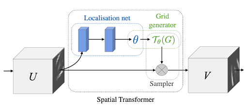
The goal of Spatial transformer networks (STN for short) is to add to your base network a layer able to perform an explicit geometric transformation on an input. STN is a generalization of differentiable attention to any spatial transformation. It allows a neural network to learn how to perform spatial transformations on the input image to enhance the geometric invariance of the model.
The layer is composed of 3 elements:
- The localization network takes the original image as an input and outputs the parameters of the transformation we want to apply.
- The grid generator generates a grid of coordinates in the input image corresponding to each pixel from the output image.
- The sampler generates the output image using the grid given by the grid generator.
The given dataset shows that the traffic signs were taken at a wide variety of angles and distances. So we preprocessed the input image by the Spatial Transformer Networks.
We start by splitting the data into train and validation sets with a train to validation ratio of 4:1 and with a batch size of 64. We do not apply any fancy image augmentations but all the train and validation images are resized to 32x32 pixels and normalized to a mean of [0.3401,0.3120,0.3212] and a standard deviation of [0.2725,0.2609,0.2669] which were calculated on a train set of images.
We used Adam optimizer with a learning rate of 0.001 and Cross-Entropy Loss as the criterion. The baseline models were trained on using the above-mentioned model and regularisation parameters for a few hundred epochs.
We use the same baseline model as stated above but with a few changes to training a model on uploaded images.
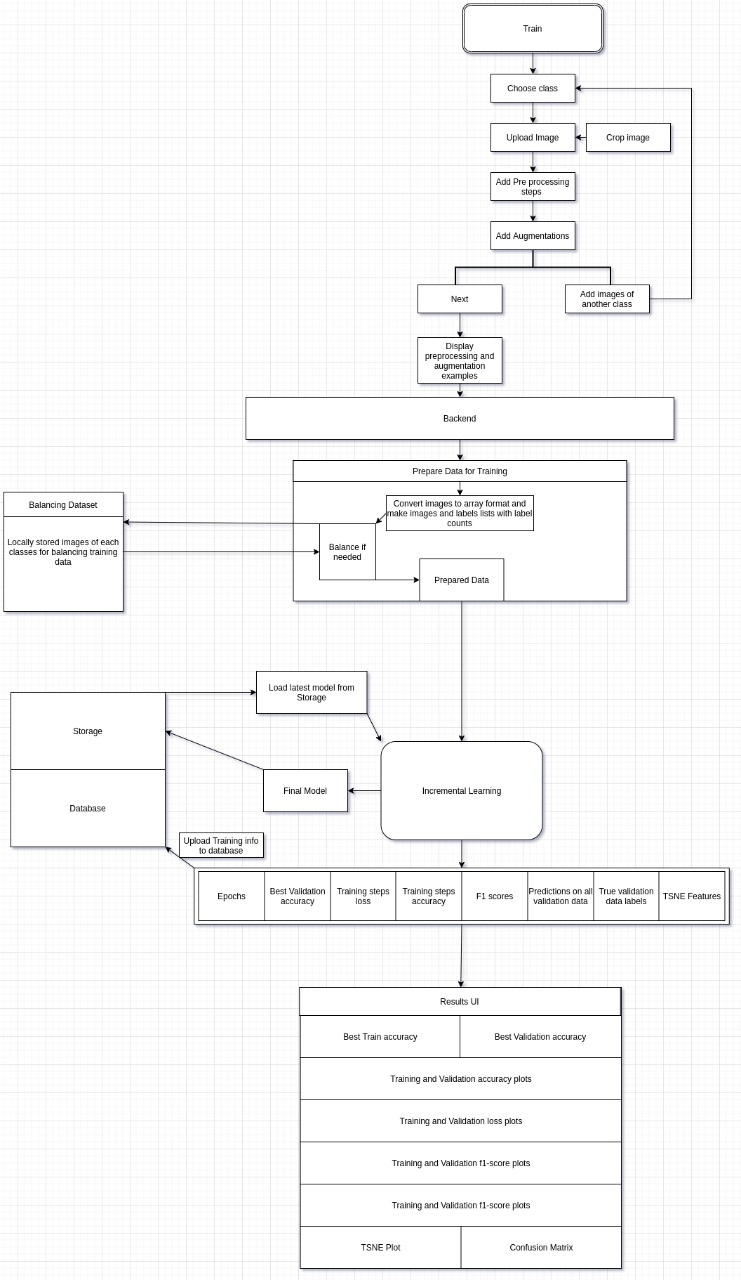
Training a new model every time the user uploads a new set of images is time-consuming and there may not be a major change in how the model learns the representation of the classes. Due to our limit in resources and time, we have chosen to implement incremental learning to train on images uploaded by the user through the provided GUI.
Incremental learning is a method of machine learning in which input data is continuously used to extend the existing model's knowledge i.e. to further train the model. It represents a dynamic technique of supervised learning and unsupervised learning that can be applied when training data becomes available gradually over time or its size is out of system memory limits.
The aim of incremental learning is for the learning model to adapt to new data without forgetting its existing knowledge. We have implemented the most rudimentary way of applying Incremental learning using the principles of transfer learning.
The model is trained on only the newly uploaded images by the user with a reduced learning rate and epoch count. Through our experiments, we found out that keeping the learning rate low prevented the model from forgetting previously learnt representation of classes and reducing the epoch count to around 10%-20% of the original base model epochs, preventing the model from overfitting on the newly added images.
The preprocessing and augmentation of images will take place as directed by the user in the UI provided at the time of uploading the images and saved them in the designated folder.
The following metrics are used to interpret the model's performance :
1. Accuracy: Accuracy score gives us information directly about the model. If the score is higher than previous model's score than the changes made by user is helping the model and boosting its performance but if score decreases than the changes made by user is backfiring. In the case where accuracy score decreases the user should
- add proper regularization to the network,
- add more images for training and retrain the model.
2. Loss: If the validation loss seems to be much higher than training loss, it implies us that the model is starting to overfit on the data and hence solution the this issue would be
- to add proper regularization to the network,
- to simplify the network,
- to add more images for training and retrain the model.
3. Confusion Matrix: The Confusion Matrix helps us to understand on how well the model is performing the classification task. It provides us with the data of True Positives, True Negatives, False positives and False Negetives, which gives us a broad view on how well the model works. So if True Positives and True Negatives have compatively much higher than False Positives and False Negatives then the model is working fine else we need to imporve our model by adding images to data set and train it well on our data.
4. T-SNE Plot: The T-SNE plot represents the features in the fully connected layers of the neural network which our network learns in 2 dimensions. So if datapoints in the plot for different classes are seen to be not localized properly, it implies us that the model finds it difficult to learn distinguishing features for those classes. Hence the solution is to add more images of these classes and retraining the model with extended dataset.
5. F1-Score: F1 Score is an overall measure of the model's accuracy. A good score implies that the model trained has lower number of False Positives and False Negetives. If the F1 score decreases then the recent changes made to the model is effecting the model in negetive way. Hence in such case to imporve the model we should add more images for training and retrain the model.
6. Saliency Map: Deep learning models are often thought of as black-boxes, making them difficult to interpret and debug. The saliency map shows the pixel-wise importance of an image to the neural network trained on it. The higher the importance of the pixel in helping classify the image, the brighter the colour of the pixel in the saliency map. The saliency map helps us understand how the deep learning model sees the input image and whether the image features are captured correctly or not. Thus if the localisation in the Saliency Map is not around the road sign in the image it means that the model isn't learning to classify the image and some kind of bias in the data is effecting its performance. Thus as solution to improve the model could be that we could add more images of the class of the image whose saliency map isn't accurate and is biased in some way so that model can understand the bias and negate its effect.
In order to run the project, your machine will need to download few things to set the enviroment and avoid any breakdowns while running.
1. Download npm. You can download npm along with nodejs according to your os from here: https://nodejs.org/en/download/
To check if it has downloaded run the following command:
npm --versionIf it shows the version number then you have successfully downloaded npm.
2. Download Yarn package manager through npm. Run the following command in your terminal:
npm install --global yarn3. Install git according to your os from here:
https://git-scm.com/book/en/v2/Getting-Started-Installing-Git
1. Clone this repo
git clone https://github.com/dhritimaandas/Traffic_Sign_Recog_Inter_IIT.git
cd Traffic_Sign_Recog_Inter_IIT/ui2. Now since you are in the root directory for the Next.Js project, install the required packages.
yarn install3. Now run the development server.
yarn devOpen http://localhost:3000 with your browser to see the result.
Replace the firebaseConfig file with your own config file in Traffic_Sign_Recog_Inter_IIT/backend/config/
1. Clone this repo using
git clone https://github.com/dhritimaandas/Traffic_Sign_Recog_Inter_IIT.git2. Navigate to working directory and then to backend folder using
cd backend3. Make sure you have installed pipenv. If not run the command
pip install pipenv4. Spawn a new virtual environment
pipenv shell5. Download all the dependencies
pipenv install6. To run flask app execute
python app.pyChoose a class from the given options and add images through the "Add Images" button.
You can crop your images with the shown crop button
After cropping the image you will see a side-by-side comparison of the original and the cropped image.
You can add several preprocessing techniques to your images as shown
You can add augmentations to your images as shown. After clicking on next you will be redirected to the the page showing the final images sent to model.
You can check the final images sent here and if you don't like feel free to reset your progress.
You can balance and spilt the dataset from here.
Note: Make sure you have integrated the firebase to the backend for the model to work. Refer Setting up Firebase.
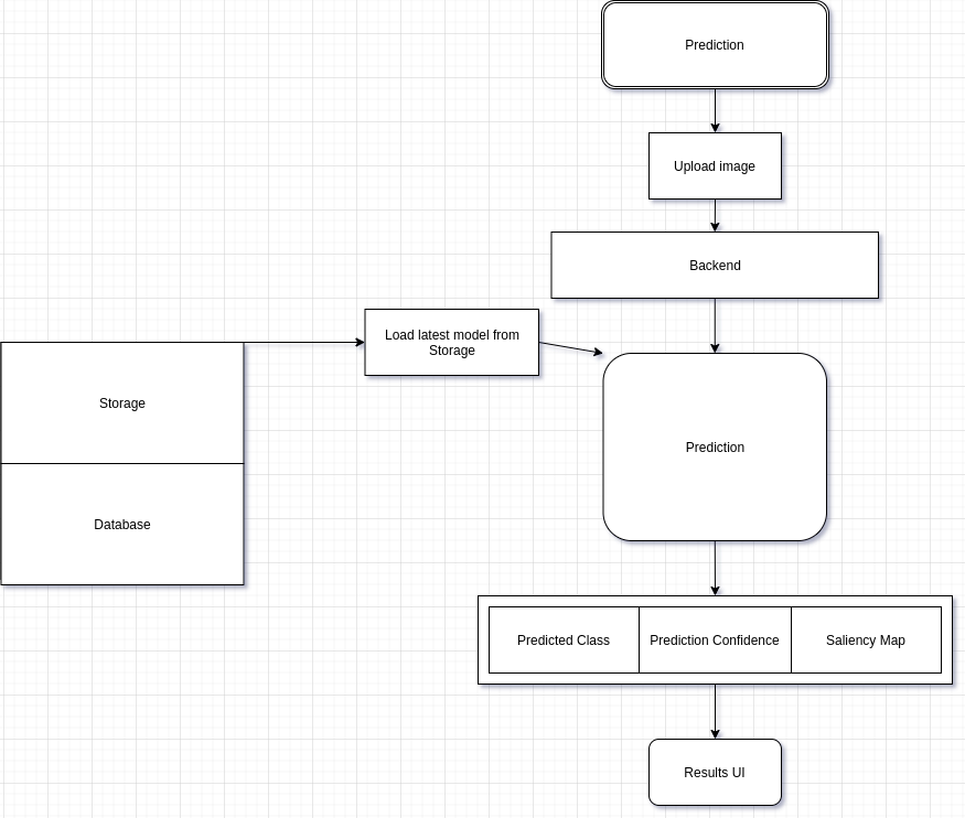
You can add a image to predict its class as shown.
Note: Make sure you have integrated the firebase to the backend for the model to work. Refer Setting up Firebase.
You will see the result as shown above. You will also be able to see a saliency map. A saliency map is an image that shows each pixel's unique quality. The aim of saliency map is to simplify and/or change the representation of an image into something that is more meaningful and can be used to analyze how the model reads the image and what features are important for making the prediction.
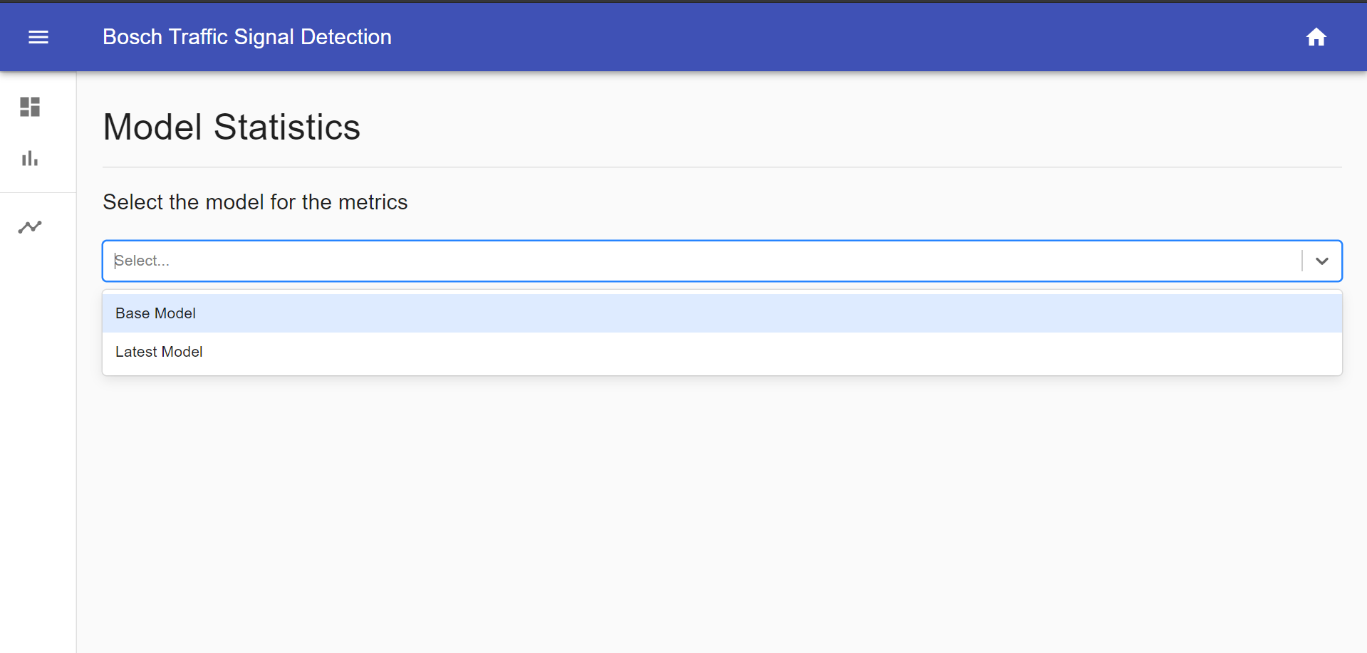
You can select the model from the menu as shown.
You will be also be given some information about how can you improve your model. You can access it by clicking How to improve my model?.
- You can select the Model for which you want to analyse the metrics.
- Here you can have access to various information like Training Accuracy and Validation Accuracy along with their line-charts.
- The user is shown a discrete graph plot of T-SNE Data.
- There is a Confusion Matrix to analyse and study. -You can
- The user can determine Training and Validation Loss and their F1 Score through their separate line-charts.
- You can over at any point of Confusion Matrix or any other chart to view the statistics of that particular coordinate.
- You can toggle the the view of line-charts to focus on other information by clicking on the legend as shown below:
.png)
.png)
.png)
.png)
.png)
.png)
.png)
.png)
.png)
.png)
.png)
