windR is a R package to connect animal tracking data with wind data
(or sea current data) and allows to visualize animal movements within
the flow of the medium that they moved in.
The package was written to compile functions used to analyse pectoral sandpiper movements in the wind. A full animation of these tracks can be found on youtube: Moving though the Arctic: Pectoral sandpipers in the wind
windR uses wind data from
ERA-Interim
(a global atmospheric reanalysis model) described in detail in Dee et
al. 2011
and connects them wind tracking data (your own). It can be used to
create particle flow animations of wind or sea current data. To connect
them with tracking data, it is necessary to calculate the bearing
(ground direction), ground speed, wind support and cross winds from
animal tracks using an equal area map projection (e.g.Lambert azimuthal
equal-area
projection).
The wind support represents the length of the wind vector in the
direction of the birds’ flight and the cross wind represents the length
of the wind vector perpendicular to ground vector (see Safi et
al. 2013
for schematic
representation).
For a detailed description see the workflow example described below.
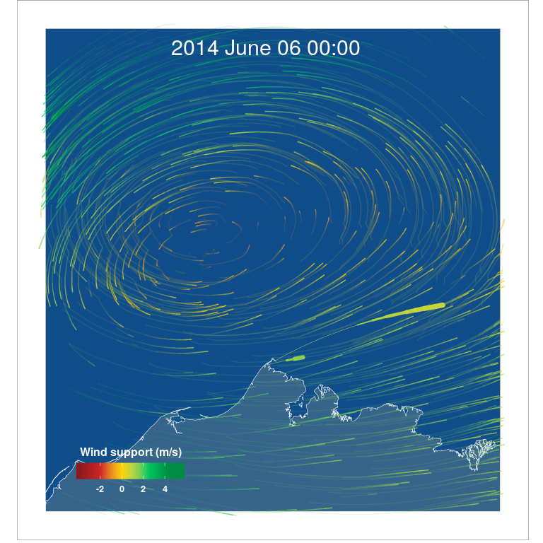
The figure shows an example snapshot of the particle flow animation including two male Pectoral Sandpipers (thick comets in light green) that left the area around Barrow (northern tip of Alaska) coloured with the wind support (m/s) and wind particles coloured with the wind speed (m/s; same scale as wind support) flying around based on the wind data at this time. Map projection: polar Lambert azimuthal equal-area with longitude origin 156.65° W (Barrow); Map data from Natural Earth
The vignettes give a small step by step example of what one has to do to reach the final result (a particle flow animation with animal tracks). The single vignettes are built up on each other, but each can be run independently (since the output data of each step can be loaded from the package data). The vignettes as html can be found at OSF and viewed in a browser after downloading.
The first vignette A_ERA_Interim_data_download describes how to download the ERA-Interim data using a python script. Note that single month can also be downloaded via the website directly.
The second vignette B_Wind_data_manipulation describes how to open the wind data, interpolate them to a higher resolution and transform them in a data.table including the date and u- & v-wind component.
The third vignette C_Wind_particle_flow describes on how to use wind data to calculate a particle flow (how to create particles) and how to create an animation with them.
The forth vignette D_Wind_support_and_track_animation describes how to connect animal tracks (using a subset of data from Kempenaers & Valcu 2017) with wind data and how to calculate the bearing, ground speed, wind support and cross winds from the tracks. Afterwards, it gives an example of how to plot the tracking data in a simple ggplot and how to do a comet plot animation using tracking data.
The fifth vignette F_Wind_animation_with_tracks brings everything together. It combines the particle flow animation of the wind data with the tracking data.
- Follow the vignettes and run the examples.
- Start small with your own data! Take a small subset of your data to go thru the whole process (of whatever you want to do). Starting with a big data set makes everything slow and will make you soon frustrated. If everything is as you which with your small subset – go big and create particles for the whole period of your interest.
- Find the optimal spatial and temporal scale fitting to your tracking data and question.
- Have fun!
install.packages('devtools')
devtools::install_github('mpio-be/windR')

# install with vignettes
devtools::install_github("mpio-be/windR", build_vignettes = TRUE, force = TRUE)
vignette(package = "windR")All analyses are constrained by the spatio-temporal resolution of the used wind and tracking data.
This project was inspired by the awesome earth project from Cameron Beccario, which was itself inspired by the wind map project from HINT.FM.
We saw these particle flow maps of the wind and wanted to see our bird
tracks within such a visualization. Both earth and wind map use
fixed times of global wind data sets (one wind layer). Particles are
randomly thrown in the map and move based on the wind speed and
direction. To plot our bird tracks within the wind, we needed to find a
way to continuously change the wind data with the time that the birds
moved. We did so by always using the closest wind data in time
(continuously changing the wind layers), resulting in a dynamic flow of
the wind particles changing over time. We did our best to make this
workflow fast in R, but know that using other programming languages
(i.e. JavaScript) could improve the speed of these analyses. We are
happy if somebody wants to improve (speed-up) this script or translates
parts (esp. the particle creation) into another programming language.


