Kolmogorov-Arnold Networks (KAN)

A 2024 Alternative to Multi-Layer Perceptrons with Learnable Activation Functions

Project Overview

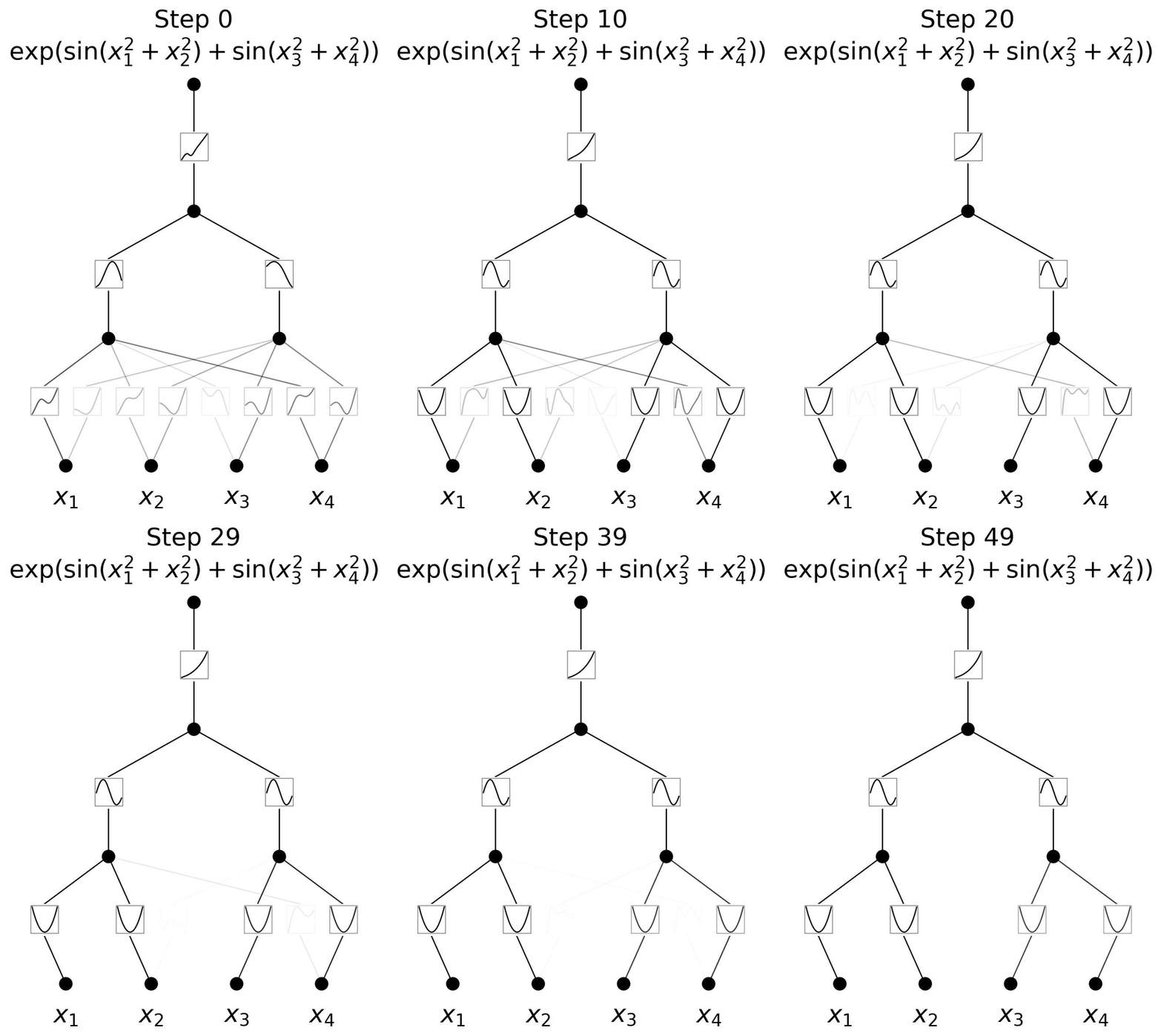
Developed in 2024, Kolmogorov-Arnold Networks (KANs) are inspired by the Kolmogorov-Arnold representation theorem and represent a significant evolution from traditional Multi-Layer Perceptrons (MLPs). In MLPs, nodes ("neurons") have fixed activation functions. However, in KANs, activation functions are learnable and applied to the edges (weights), allowing the network to dynamically adjust and learn more complex functions.

KANs eliminate linear weights, replacing them with univariate functions parameterized as splines. This architectural change makes KANs both more accurate and more interpretable than standard MLPs. They are also smaller in size, making them efficient for a wide range of tasks, including data fitting and solving partial differential equations (PDEs).

Kolmogorov-Arnold Networks vs. MLPs

Learnable Activation Functions: Unlike MLPs, where activation functions are fixed (e.g., ReLU, Sigmoid), KANs have dynamic, learnable activation functions placed on the edges (weights).
Spline-Based Weights: KANs do not use traditional linear weights. Instead, each weight is replaced by a univariate function, which allows the network to learn more sophisticated representations.
Smaller Network Size: KANs can achieve comparable or better accuracy than MLPs with a significantly smaller number of parameters, leading to better efficiency in both memory and computation.
Interpretability: The functional form of the weights can be visualized, allowing KANs to offer intuitive insights into how the network learns and operates.

Key Features

Learnable Activation Functions on Weights: Provides greater flexibility compared to fixed activations on neurons.
No Linear Weights: Weights are modeled as splines (univariate functions), enabling a more sophisticated representation of the underlying data.
Higher Accuracy: Smaller KANs can outperform larger MLPs in a variety of tasks, including mathematical modeling and physics simulations.
Visualizable and Interpretable: The structure of KANs can be intuitively visualized, allowing easy interaction with users to understand the inner workings of the network.
Applications: Useful for data fitting, solving PDEs, and potentially (re)discovering mathematical and physical laws.

Installation

To run the Kolmogorov-Arnold Networks (KAN) project locally, follow these steps:

Clone the repository:

git clone https://github.com/your-username/kan-implementation.git

Navigate to the project directory:
```
cd kan-implementation
```
Install the required dependencies:
```
pip install -r requirements.txt
```
The key dependencies include:
- torch (PyTorch)
- graphviz
- matplotlib

Usage

Once the dependencies are installed, you can experiment with the KAN model by running the provided scripts.

Example Usage:

Define the KAN model and dataset:

input_size = 2
layer_sizes = [2, 2, 2, 1]
kan = KAN(input_size, layer_sizes)

Train the KAN model:

x = [[Tensor(0.25), Tensor(0.25)], [Tensor(0.25), Tensor(0.75)], [Tensor(0.75), Tensor(0.25)], [Tensor(0.75), Tensor(0.75)]]
y = [0.25, 0.75, 0.75, 0.25]

n_epochs = 100
optim = Optimizer(lr=0.001)

for _ in range(n_epochs):
    losses = Tensor(0)
    for _x, _y in zip(x, y):
        y_hat = kan(_x)
        loss = compute_loss(y_hat, _y)
        losses = loss + losses
    
    optim.zero_grad(kan.parameters())
    losses.grad = 1
    losses.backward()
    optim.step(kan.parameters())

Visualize the computational graph:
```
draw_dot(y_hat)
```

Training the Model

The KAN model can be trained by feeding input and output pairs and optimizing the weights using the gradient descent method. This project provides an Optimizer class for backpropagation and gradient updates.

Example Training Loop:

for _ in range(n_epochs):
    losses = Tensor(0)
    for _x, _y in zip(x, y):
        y_hat = kan(_x)
        loss = compute_loss(y_hat, _y)
        losses = loss + losses

    optim.zero_grad(kan.parameters())
    losses.grad = 1
    losses.backward()
    optim.step(kan.parameters())

mr-seifi/kan-implementation