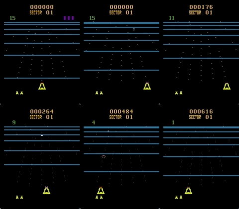
TensorFlow implementation of asynchronous advantage actor-critic (A3C) for Atari games using OpenAI Gym, built with love, kindness - and since deep RL is apparently easy to mess up - OCD levels of thoroughness and care.
The main Atari games tested in the paper were Beamrider, Breakout, Pong, Q*bert and Space Invaders. Reported results on A3C (Figure 4) from the paper were:
OCD A3C achieves comparable results on Pong and Breakout; superior results on Q*bert; but significantly worse results on Beamrider and Space Invaders:
(Original logs for these runs, commands used to run them, resulting policies, and script used to plot results can be found at ocd-a3c-runs/master_a19cf29.)
I'm assuming discrepancies are due to hyperparameter differences: the paper tries 50 different learning rates/initializations for each game and reports the best three, whereas our results use the same hyperparameters throughout: learning rate 1e-4 and a gradient clip of 5.0 (with shaded regions showing best/worst scores over three random seeds).
How close to a linear speedup do we get from adding extra workers?
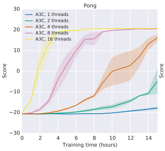
The most dramatic results from the paper were for Pong:
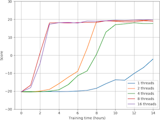
Running on 16 cores, though OCD A3C does match the performance for 16 workers, the speedups between 1 and 16 workers are not as linear:
(Data for these runs can be found at ocd-a3c-runs/master_60d4b42.)
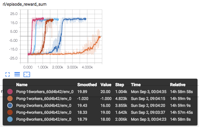
However, the speedup does seem to be roughly linear when scores are instead plotted against episode number:
This suggests that OCD A3C functions correctly in terms of accelerating learning by aggregrating experience from multiple workers, but just that there's overhead from extra workers due to e.g. GIL (described below).
To set up an isolated environment and install dependencies, install
Pipenv (e.g. pip install --user pipenv), then just run:
$ pipenv sync
However, note that TensorFlow must be installed manually. Either:
$ pipenv run pip install tensorflow
or
$ pipenv run pip install tensorflow-gpu
depending on whether you have a GPU. (If you run into problems, try TensorFlow 1.10.)
If you want to run tests, also run:
$ pipenv install --dev
Finally, before running any of the scripts, enter the environment with:
$ pipenv shell
We support Atari environments using a feedforward policy. Basic usage is:
$ python3 train.py --n_workers <no. of workers> <environment name>
For example, to train an agent on Pong using 16 workers:
$ python3 train.py --n_workers 16 PongNoFrameskip-v4
TensorBoard logs and checkpoints will be saved to a new directory in runs. To specify the name of
the directory, use --run_name.
Run train.py --help to see full usage options, including tuneable hyperparameters.
Once training is completed, examine trained behaviour with:
$ python3 run_checkpoint.py <environment name> <checkpoint directory>
For example, using a checkpoint from ocd-a3c-runs:
$ python3 run_checkpoint.py PongNoFrameskip-v4 ocd-a3c-runs/Pong-0_a19cf29/checkpoints/
Tests can be run individually, e.g.:
$ tests/network_test.py
Or all together, with:
$ python3 -m unittest tests/*_test.py
To earn its epithet, OCD A3C includes a few special testing features.
An annoying thing with deep RL is when a change which should be inconsequential apparently
breaking things because it inadvertently changes random seeding. To make it more obvious when this
might have happened, train_test.py does an end-to-end run starting
from a fixed seed, checking that after 100 updates on a deterministic environment,
weights are exactly the same as what they were in previous versions of the code.
Run preprocessing_play.py to play the game through the eyes of the agent using Gym's
play.py.
You'll see the full result of the preprocessing pipeline (including the frame stack, spread out
horizontally over time):
Still, what if we fumble something up between the eyes and the brain - between the preprocessing pipeline and actually sending the frames into the policy network for inference or training?
Using tf.Print, we can dump all data
going into the network then later check whether things are right. This involves first running
train.py with the --debug flag and piping stderr to a log file:
$ python3 train.py PongNoFrameskip-v4 --debug 2> debug.log
Then, run show_debug_data.py on the resulting log:
$ python3 show_debug_data.py debug.log
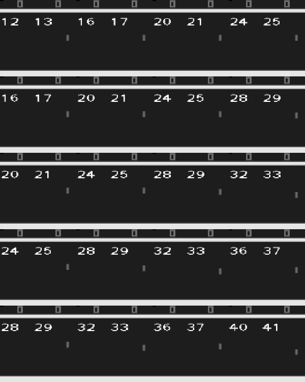
You'll see the first five four-frame stacks used to choose actions on the first five steps in the environment (with individual frames numbered - starting from 12 here because of the random number of initial no-ops used to begin each episode - and with two numbers on each frame because of the maximum taken over subsequent frames):
Then the stack from the final state reached being fed into the network for value estimation:
Then a batch of the first five stacks all together, used for for the first training step:
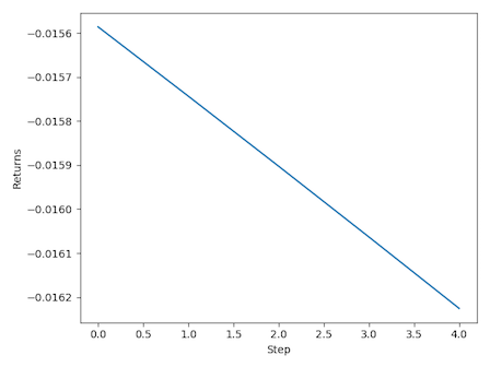
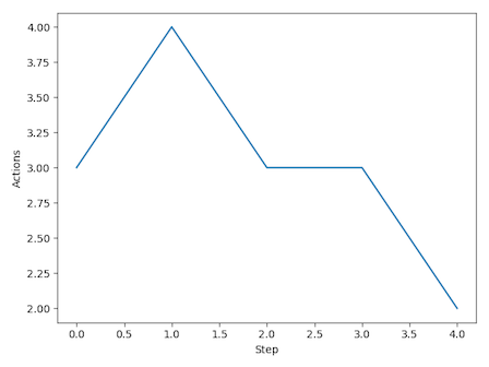
With the corresponding returns and actions for the training batch:
Then the stack from the current state being fed into the network again to choose the first action of the next set of steps:
And so on.
The initial design ran each worker on a separate process, with replication of shared parameters done
using Distributed TensorFlow. I hoped that, avoiding global interpreter lock, this would be the
fastest way to do it, but the replication seemed to have a large overhead - it actually turned out
to be faster to run the workers on threads, so that no replication is necessary, running only the
environments in separate processes. This was inspired by OpenAI Baselines'
SubprocVecEnv.
How does OCD A3C's training throughput (environment steps/second) compare to a reference implementation?
On a 16-core machine (an EC2 c5.4xlarge), running 16 workers:
- A2C from OpenAI Baselines achieves ~1000 steps per second
- OCD A3C achieves ~500 steps per second
The reduced through compared to A2C is presumably due to some combination of:
- The need for each worker to synchronise its own copy of the network with the global network on every update.
- Gradients being computed for each worker's batch of experience separately, rather than being able to compute gradients on one large batch combining the experience from all workers at once, as in A2C.
- GIL-induced thread juggling, since each worker runs on a separate thread.
A nice thing about A3C is that there are lots of other implementations. Check out how other people have implemented the same thing:
- OpenAI's universe-starter-agent
- Denny Britz's implementation in his reinforcement-learning repo
- Yasuhiro Fujita's async-rl
- Kosuke Miyoshi's async_deep_reinforce
- (Bonus 1: NVIDIA's GA3C, which uses a slightly different architecture but might be interesting nonetheless)
- (Bonus 2: OpenAI's A2C implementation)
Thorough archival of test runs is absolutely vital for debugging. (I talk a bit more about this in the context of a a different paper at Lessons Learned Reproducing a Deep Reinforcement Learning Paper.)
Using a managed service like FloydHub is nice if you can afford it, but for this implementation I was mainly using my university's cluster. The DIY solution I converged on by the end of this project was the following:
- Store runs in a separate repository (so that when you're copying the code to a new machine you don't also have to copy all the runs), under Git LFS. (Example: ocd-a3c-runs.)
- Maintain a separate branch in that repository for each revision in the main code repository you do runs from, labelled by branch.
- Have your code automatically label each run with the current revision, just in case you mess up the branches. (See e.g. params.py.)
- Save the arguments used for each run - both those specified on the command line, and the full
e.g.
argparsenamespace so you record default arguments too (also params.py).
Preprocessing of Atari environment frames was by far the hardest thing to get right in this implementation. Over the course of the project I ended up reimplementing preprocessing two times before it was in a form I was confident was correct and was easily testable.
The final solution is heavily inspired by OpenAI Baselines'
atari_wrappers.
Taking a layered approach to preprocessing, with each stage of preprocessing being done using a
separate wrapper, makes both implementation and testing a lot easier.
If you're reproducing papers to learn about deep RL, I strongly recommend just using
atari_wrappers. Implementing the preprocessing from scratch did give me a much stronger
appreciation for the benefits of layered design, and it seems important to know about the tricks
that are used (episode reset on end-of-life and no-ops at the start of each episode came as
particular surprises to me), but it takes away so much time that could be spend learning about
actual RL stuff instead.
At the start, I was thinking that Monte Carlo updates would be simpler to get working than the 5-step temporal difference updates suggested by the paper - the bias introduced by the value bootstrap seemed like it might complicate things. But during initial testing on Pong, though MC updates did work when using heavy preprocessing (removing the frame and background, and setting the ball and paddles to pure white), MC updates didn't work at all when using the generic Atari preprocessing (just resizing and grayscaling the frame).
The ostensible explanation is that MC updates are much higher variance and therefore take longer to converge. Maybe training was just too slow to show significant progress on the length of the runs I was doing (~ 12 hours). But I'm hesitant to accept this as the full explanation, since MC updates worked fine with the heavier preprocessing, and without taking too much longer.
Another possible explanation is the difference in gradient accumulation/updates between MC and TD. The pseudocode in the paper suggests simply summing gradients over each step. With MC updates, because you're summing gradients over the many steps of an entire episode, you'll end up taking a really large step in parameter space on every update. Updates that large just seem like a bad idea. You could limit the size of the updates by e.g. dividing by the number of steps per episode, but then you're going to be learning much more slowly than with TD updates, where you're also making only small updates but you're making them much more regularly.
It's still surprising that large MC updates work at all with the heavier preprocessing, though. Maybe it's something to do with the sparsity of the observations, zeroing out everything but the ball and paddles. But I never did completely figure this out.
In summary: even though MC updates might seem conceptually simpler, in practice MC updates can work a lot worse than TD updates; and in addition to the standard bias/variance tradeoff explanation, I suspect it might be partly that with MC updates, you're taking large steps infrequently, whereas with TD updates, you're taking small steps more frequently.
One explanation for why running multiple workers in parallel works well is that it decorrelates updates, since each worker contributes different experience at any given moment.
(Note that Figure 3 in the paper suggests this explanation might apply less to A3C than the paper's other algorithms. For A3C the main advantage may just be the increased rate of experience accumulation. But let's stick with the standard story for now and see where it goes.)
Even if there's diversity between each update, though, this says nothing about the diversity of experience within each update (where each update consists of a batch of 5 steps in the environment from one worker). My impression from inspecting gradients and RMSprop statistics here and there is that this can cause problems: if each update is too homogenous, each update can point in one direction kind of sharply, leading to large gradients on each update. Gradient clipping therefore seems to be pretty important for A3C.
(I didn't experiment with this super thoroughly, though. Looking back through my notes, gradient norms and certain RMSprop statistics were definitely different with and without gradient clipping, sometimes up to a factor of 10 or so. And I do have notes of some runs failing apparently because of lack of gradient clipping. Nonetheless, take the above story with a grain of salt.)
(Also note that this is in contrast to A2C, where each update consists of experience from all workers and is therefore more diverse.)
Sadly, amount of gradient clipping is one hyperparameter the paper doesn't list (and in fact,
learning rate and gradient clipping were tuned for each game individually). The value we use
(max_grad_norm in params.py) of 5.0 was determined through coarse line search over
all five games.
My main thoughts from these experiences are:
- If you're calculating gradients on batches with correlated data, gradient clipping probably is something you're going to have to worry about.
- If you use gradient clipping in your paper, please quote what clip value you use.
Overall, this project took about 150 hours. That's much longer than I expected it to take.
I think the main mistake I made was starting from a minimal set of features and gradually adding the bells and whistles rather than starting from a known-good implementation then ablating to figure out what was actually important. Some of the extras do end up just being small performance improvements, but sometimes they're the difference between it working fine and not working at all, and it can be really hard to guess in advance which any particular feature will be. (I'm thinking in particular about a) gradient clipping and b) the difference between MC updates and TD updates. To my unexperienced self at the start of the project, both of these seemed like completely reasonable simplifications. But figuring out that these two were key took so, so much time - there were always other bugs which were easier to find and initially seemed important but once fixed turned out to be non-critical red herrings.)
Advice I've since heard for how to approach these reproductions more efficiently instead suggests a process more like:
- Start with an existing implementation from a trusted source.
- Scrutinize the code and experiment with small parts of it until you're confident you understand what every single line does. Make notes about the parts you're suspicious about the purpose of.
- Rewrite the same implementation basically verbatim from memory. Test, and if it fails, compare to the original implementation. Iterate until it works.
- Start again from scratch, writing an implementation in your own style. Once it works, ablate the parts you were suspicious of.


