simrabid is an implementation of a spatially explicit,
individual-based model of canine rabies. It is very much a work in
progress!
And the development version from GitHub with:
# install.packages("devtools")
devtools::install_github("mrajeev08/simrabid")

# To install suggested packages & dependencies:
devtools::install_github("mrajeev08/simrabid", dependencies = TRUE)This is a basic example which shows you the very basics:
library(raster)
#> Loading required package: sp
library(data.table)
#>
#> Attaching package: 'data.table'
#> The following object is masked from 'package:raster':
#>
#>     shift
library(sf)
#> Linking to GEOS 3.8.1, GDAL 3.1.4, PROJ 6.3.1
library(tidyr)
#>
#> Attaching package: 'tidyr'
#> The following object is masked from 'package:raster':
#>
#>     extract
library(dplyr)
#>
#> Attaching package: 'dplyr'
#> The following objects are masked from 'package:data.table':
#>
#>     between, first, last
#> The following objects are masked from 'package:raster':
#>
#>     intersect, select, union
#> The following objects are masked from 'package:stats':
#>
#>     filter, lag
#> The following objects are masked from 'package:base':
#>
#>     intersect, setdiff, setequal, union
library(magrittr)
#>
#> Attaching package: 'magrittr'
#> The following object is masked from 'package:tidyr':
#>
#>     extract
#> The following object is masked from 'package:raster':
#>
#>     extract
library(simrabid)
library(ggplot2)

# Use the example serengeti shapefile in the package
sd_shapefile <- st_read(system.file("extdata/sd_shapefile.shp",
                                    package = "simrabid"))
#> Reading layer `sd_shapefile' from data source `/Library/Frameworks/R.framework/Versions/4.0/Resources/library/simrabid/extdata/sd_shapefile.shp' using driver `ESRI Shapefile'
#> Simple feature collection with 75 features and 12 fields
#> geometry type:  POLYGON
#> dimension:      XY
#> bbox:           xmin: 637186.6 ymin: 9754400 xmax: 707441.9 ymax: 9837887
#> projected CRS:  WGS 84 / UTM zone 36S

# 1. set up the space at 1000m res
sd_shapefile$id_col <- 1:nrow(sd_shapefile)
out <- setup_space(shapefile = sd_shapefile, resolution = 1000, id_col = "id_col",
                   use_fasterize = TRUE)
#> Loading required package: fasterize
#>
#> Attaching package: 'fasterize'
#> The following object is masked from 'package:graphics':
#>
#>     plot
#> The following object is masked from 'package:base':
#>
#>     plot

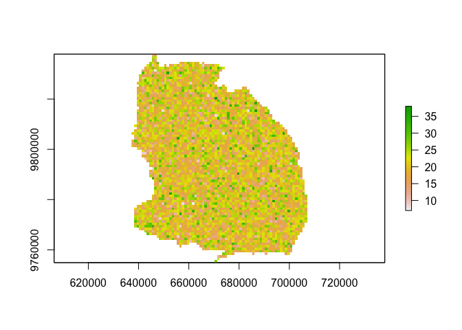
# Fake some pop data here
pop_out <- out
values(pop_out) <- rpois(ncell(pop_out), 20)
pop_out[is.na(out)] <- NA
plot(pop_out)
# 2. set-up simulation framework (timesteps + demography)
start_up <- setup_sim(start_date = "2002-01-01",
apprx_end_date = "2020-01-01",
days_in_step = 7,
rast = out,
death_rate_annual = 0.48,
birth_rate_annual = 0.52,
waning_rate_annual = 1/3,
params = list(start_pop = pop_out[]),
by_admin = FALSE)
# Set up vaccination
vacc_dt <- simrabid::sim_campaigns(locs = 1:75, campaign_prob = 0.9,
coverage = 0.7, sim_years = 20,
burn_in_years = 5,
steps_in_year = 52)
vacc_dt_none <- vacc_dt[0]
# Without vax
system.time({
test <- simrabid(start_up, start_vacc = 0.2, I_seeds = 3,
vacc_dt = vacc_dt_none,
params = c(list(R0 = 1.1, k = 1, iota = 0.25),
param_defaults),
days_in_step = 7,
observe_fun = beta_detect_monthly,
serial_fun = serial_lognorm,
dispersal_fun = dispersal_lognorm,
secondary_fun = nbinom_constrained,
incursion_fun = sim_incursions_pois,
movement_fun = sim_movement_continuous,
sequential = FALSE, allow_invalid = TRUE,
leave_bounds = TRUE, max_tries = 100,
summary_fun = return_env,
track = FALSE,
weights = NULL,
row_probs = NULL,
coverage = TRUE,
break_threshold = 0.8,
by_admin = FALSE)
}
)
#> user system elapsed
#> 5.764 0.643 6.580
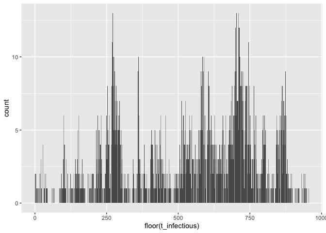
ggplot(test$I_dt) + geom_bar(aes(x = floor(t_infectious)))formals(use_mget)$names <- c("I_dt", "N_mat")
system.time({
test <- simrabid(start_up, start_vacc = 0.2, I_seeds = 3,
vacc_dt = vacc_dt,
params = c(list(R0 = 1.2, k = 1, iota = 1),
param_defaults),
days_in_step = 7,
observe_fun = beta_detect_monthly,
serial_fun = serial_lognorm,
dispersal_fun = steps_weibull,
secondary_fun = nbinom_constrained,
incursion_fun = sim_incursions_pois,
movement_fun = sim_movement_continuous,
sequential = TRUE, allow_invalid = TRUE,
leave_bounds = TRUE, max_tries = 100,
summary_fun = use_mget,
track = TRUE,
weights = NULL,
row_probs = NULL,
coverage = TRUE,
break_threshold = 0.8,
by_admin = FALSE)
}
)
#> user system elapsed
#> 9.944 1.349 11.925
# With vax
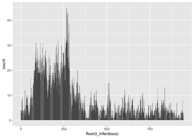
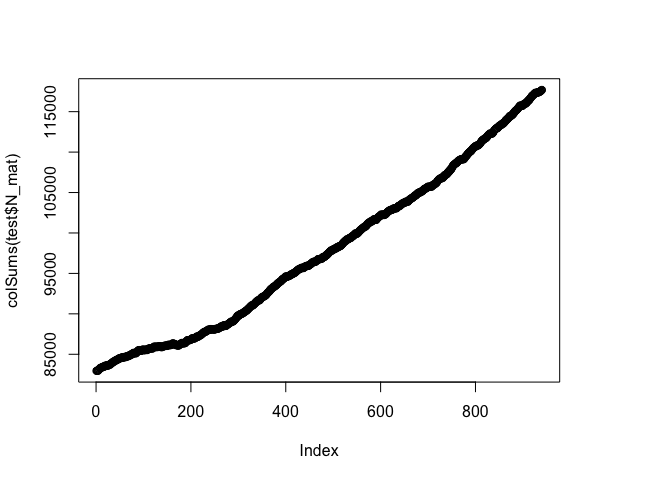
ggplot(test$I_dt) + geom_bar(aes(x = floor(t_infectious)))plot(colSums(test$N_mat))simrabid is written to be modular, feel free to poke around the
function documentation to see the options–technical vignettes coming
-
A relative probability based movement model (i.e. movement probability is relative to index location, for instance if you want to account for landscape barriers (roads, rivers, etc.)); see old commit code for how this might work with a probability list;
-
Use non utm coordinate space, instead use cellFromXY in raster and haversine distances to get location of cell id movements so that you can simulate across larger spatial scales; one issue is then your scale of aggregation gets distorted, aggregate grid cells somehow so it’s approximately 1 km?
-
Implement carrying capacity on pop growth, and replacement of dogs removed due to infection.
-
Implement colonization of uninhabited patches (with some limits so households can’t pop up in space that is uninhabitable, i.e. rivers/roads/etc.)
-
Build a constructor class that gets passed to simrabid function so that only valid combinations of model arguments can be passed, and you only have to test this once for N simulations.
-
Profile and speed up!
- Vaccination function
- Filtering data.table
- Only track currently infectious + exposed linelist
- Easy fixes (i.e. storing things in the appropriate type, keys onf filters, etc.)
-
Issue with intermediate scales where small admin units do not get matched to any grid cell
-
Village metapopulation (separate function?)
-
Example output environment for customizing summary functions
-
Applying mortality to exposed class?
-
Documentation on how to use & customize
-
Construct synthetic populations or use high res pop data to get estimates of spatial dog pops (popcompr?)
-
Benchmarks across scales, etc.
- Issue with setup_space, id col has to be numeric
- Doesn’t simulate expansion of occupied cells (i.e. colonization of patches by doggos)
- Carrying capacity for growth


