treerabid reconstructs transmission trees using line list
data–specifically in the context of contact tracing data for canine
rabies in Tanzania for the Hampson Lab.
It is still in active development and may get rehomed in the future. Before using, we highly recommend submitting an issue to this repository.
For the package used in Mancy et al/Lushasi et al.:
Or install version 1.0 from github:
devtools::install_github("mrajeev08/treerabid@v1.0", dependencies = TRUE)
Based on: - Hampson et al. 2009. Transmission Dynamics and Prospects for the Elimination of Canine Rabies.
- Cori et al. 2019. A graph-based evidence synthesis approach to detecting outbreak clusters: An application to dog rabies.
- Mancy et al. in prep.
Install from github with:
# install.packages("devtools")
devtools::install_github("mrajeev08/treerabid", dependencies = TRUE)
Dependencies: data.table, foreach, doRNG, parallel Suggests:
ggraph, ggplot2, igraph
# Dependencies for simrabid
library(raster)
library(data.table)
library(sf)
library(tidyr)
library(dplyr)
library(magrittr)
library(ggplot2)
library(fasterize)
library(lubridate)

# Additional dependencies for treerabid
library(igraph)
library(ggraph)
library(foreach)
library(doRNG)
library(doParallel)

# simrabid & treerabid
library(simrabid) # devtools::install_github("mrajeev08/simrabid")
library(treerabid)
First simulate from rabies IBM using simrabid:
# set up
sd_shapefile <- st_read(system.file("extdata/sd_shapefile.shp",
                                    package = "simrabid"))
#> Reading layer `sd_shapefile' from data source `/Library/Frameworks/R.framework/Versions/4.0/Resources/library/simrabid/extdata/sd_shapefile.shp' using driver `ESRI Shapefile'
#> Simple feature collection with 75 features and 12 fields
#> geometry type:  POLYGON
#> dimension:      XY
#> bbox:           xmin: 637186.6 ymin: 9754400 xmax: 707441.9 ymax: 9837887
#> projected CRS:  WGS 84 / UTM zone 36S

# 1. set up the space at 1000 m resolution
sd_shapefile$id_col <- 1:nrow(sd_shapefile)
out <- setup_space(shapefile = sd_shapefile, resolution = 1000, id_col = "id_col",
                   use_fasterize = TRUE)
pop_out <- out
values(pop_out) <- rpois(ncell(pop_out), 20) # fake some population data
pop_out[is.na(out)] <- NA
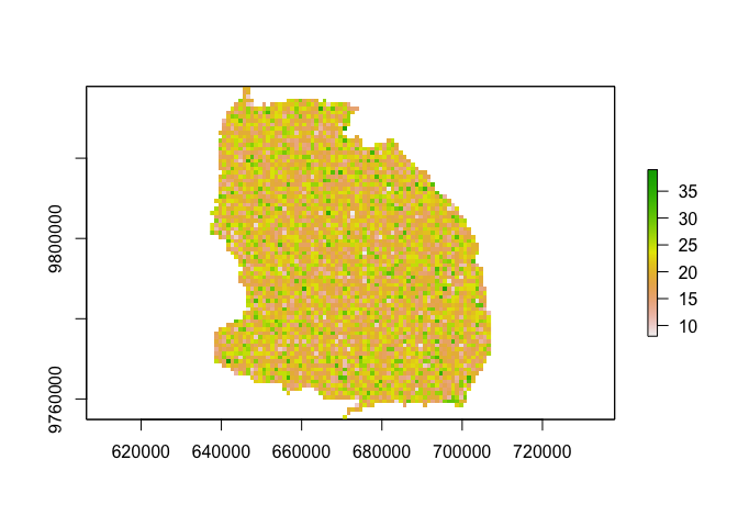
plot(pop_out)
# 2. set-up simulation framework
start_up <- setup_sim(start_date = "2002-01-01",
apprx_end_date = "2012-01-01", # apprx 10 years
days_in_step = 7, # weekly timestep
rast = out,
death_rate_annual = 0.48,
birth_rate_annual = 0.52,
waning_rate_annual = 1/3,
params = list(start_pop = pop_out[]),
by_admin = FALSE)
# 3. Simulate vaccination
vacc_dt <- simrabid::sim_campaigns(locs = 1:75, campaign_prob = 0.7,
coverage = 0.4, sim_years = 10,
burn_in_years = 0,
steps_in_year = 52)
# 4. Run the simulation
# see ?simrabid for more details on function arguments
system.time({
set.seed(1244)
exe <- simrabid(start_up, start_vacc = 0, I_seeds = 0,
vacc_dt = vacc_dt,
params = c(list(R0 = 1.1, k = 1, iota = 0.25),
param_defaults),
days_in_step = 7,
observe_fun = beta_detect_monthly,
serial_fun = serial_lognorm,
dispersal_fun = dispersal_lognorm,
secondary_fun = nbinom_constrained,
incursion_fun = sim_incursions_pois,
movement_fun = sim_movement_continuous,
sequential = FALSE, allow_invalid = TRUE,
leave_bounds = TRUE, max_tries = 100,
summary_fun = use_mget,
track = FALSE,
weights = NULL,
row_probs = NULL,
coverage = TRUE,
break_threshold = 0.8,
by_admin = FALSE)
}
)
#> user system elapsed
#> 5.753 0.526 7.237
# I_dt is the line list
case_dt <- exe$I_dt
head(case_dt)
#> id cell_id row_id progen_id path x_coord y_coord invalid outbounds
#> 1: 1 4038 2858 1 0 684947.9 9779932 FALSE FALSE
#> 2: 2 4108 2922 1 0 684816.5 9779009 FALSE FALSE
#> 3: 3 4108 2922 1 0 684679.2 9779345 FALSE FALSE
#> 4: 4 4108 2922 1 0 684609.9 9779400 FALSE FALSE
#> 5: 5 4108 2922 1 0 684479.0 9779641 FALSE FALSE
#> 6: 6 4246 3054 1 0 682803.2 9777702 FALSE FALSE
#> t_infected contact infected t_infectious month detect_prob detected
#> 1: 1.285714 S TRUE 8.963206 2 0.8790423 1
#> 2: 1.285714 S TRUE 3.914026 0 0.9165339 1
#> 3: 1.285714 S TRUE 8.320474 2 0.8790423 1
#> 4: 1.285714 S TRUE 4.546957 1 0.9087506 1
#> 5: 1.285714 S TRUE 2.000000 0 0.9165339 1
#> 6: 1.285714 S TRUE 18.801937 4 0.8732138 1Reconstruct bootstrapped trees (per Hampson et al. 2009) & prune any unlikely case pairs based on the distribution of distances between cases and a pecentile cutoff (see Cori et al):
# turn time step to dates
case_dt$date <- as_date(duration(case_dt$t_infected, "weeks") + ymd(start_up$start_date))
# construct one tree
ttrees <-
  boot_trees(id_case = case_dt$id,
             id_biter = 0, # we don't know the progenitors
             x_coord = case_dt$x_coord,
             y_coord = case_dt$y_coord,
             owned = 0,
             date_symptoms = case_dt$date,
             days_uncertain = 0,
             use_known_source = FALSE,
             prune = TRUE,
             si_fun = si_gamma1,
             dist_fun = dist_weibull1,
             params = params_treerabid,
             cutoff = 0.95,
             N = 1,
             seed = 105)
#> Warning: executing %dopar% sequentially: no parallel backend registered
ttrees2 <-
  boot_trees(id_case = case_dt$id,
             id_biter = 0, # we don't know the progenitors
             x_coord = case_dt$x_coord,
             y_coord = case_dt$y_coord,
             owned = 0,
             date_symptoms = case_dt$date,
             days_uncertain = 0,
             use_known_source = FALSE,
             prune = TRUE,
             si_fun = si_gamma1,
             dist_fun = dist_weibull1,
             params = params_treerabid,
             cutoff = 0.95,
             N = 1,
             seed = 105)

# Are these reproducible?
identical(ttrees, ttrees2)
#> [1] TRUE

# Lets do 100 trees and vizualize them
system.time({
  ttrees <-
        boot_trees(id_case = case_dt$id,
                   id_biter = 0, # we don't know the progenitors
                   x_coord = case_dt$x_coord,
                   y_coord = case_dt$y_coord,
                   owned = 0,
                   date_symptoms = case_dt$date,
                   days_uncertain = 0,
                   exclude_progen = FALSE,
                   use_known_source = FALSE,
                   prune = TRUE,
                   si_fun = si_gamma1,
                   dist_fun = dist_weibull1,
                   params = params_treerabid,
                   cutoff = 0.95,
                   N = 100,
                   seed = 105)
})
#>    user  system elapsed
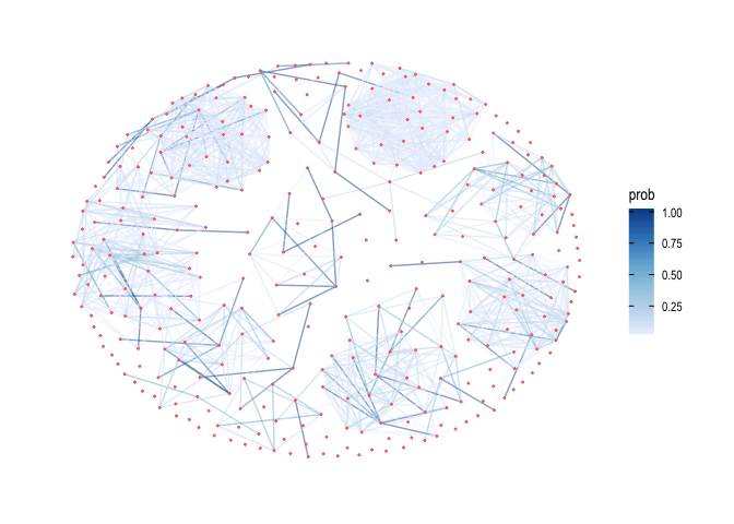
#> 5.165 0.214 6.493We can then visualize the potential links:
links_all <- build_all_links(ttrees, N = 100)
links_gr <- graph_from_data_frame(d = data.frame(from = links_all$id_progen,
                                                 to = links_all$id_case))
#> Warning in graph_from_data_frame(d = data.frame(from = links_all$id_progen, : In
#> `d' `NA' elements were replaced with string "NA"
E(links_gr)$prob <- links_all$prob
V(links_gr)$membership <- components(links_gr)$membership

# Get rid of the NA links (i.e. differentiating incursions)
links_gr <- delete_vertices(links_gr, names(V(links_gr)) %in% "NA")

set.seed(179)
ggraph(links_gr, layout = "kk") +
  geom_edge_link0(aes(col = prob), alpha = 0.5) +
  geom_node_point(aes(col = factor(membership)), size = 0.3) +
  scale_color_discrete(guide = "none") +
  scale_edge_color_distiller(direction = 1) +
  theme_graph()
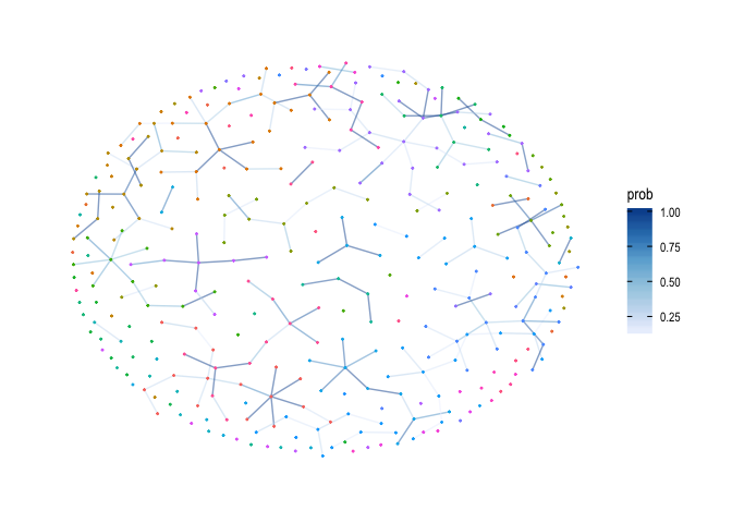
Visualize the consensus links and how certain they are:
# get the time!
links_consensus <- build_consensus_links(links_all,
                                         case_dates = case_dt[, .(id_case = id,
                                                                  symptoms_started = date)])
cons_gr <- get_graph(from = links_consensus$id_progen,
                     to = links_consensus$id_case,
                     attrs = case_dt[, .(id_case = id,
                                         t = 0)])
E(cons_gr)$prob <- links_consensus[!is.na(id_progen)]$prob
V(cons_gr)$membership <- components(cons_gr)$membership

set.seed(145)
# color incursions by membership + alpha = their probability
ggraph(cons_gr, layout="kk") +
  geom_edge_link0(aes(col = prob), alpha = 0.5) +
  geom_node_point(aes(col = factor(membership)),size = 0.3) +
  scale_edge_color_distiller(direction = 1) +
  scale_color_discrete(guide = "none") +
  theme_graph()
Incursions are those that didn’t have any potential progenitor within the cutoff time & distance. We can see the probability for each case being an incursion (total and for those that were assigned as such) (actually this is always one because not any uncertainty in dates!)
incs_all <- links_all[is.na(id_progen)]

ggplot(incs_all) +
  geom_histogram(aes(x = prob))
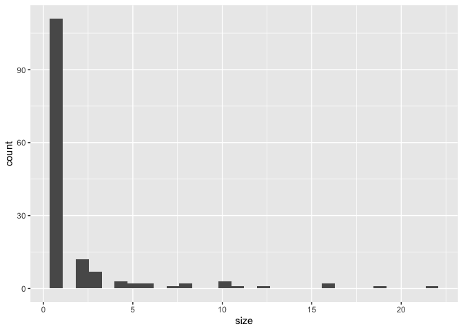
Compute chains stats on the consensus links:
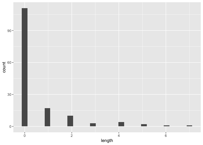
chain_stats <- get_chain_stats(cons_gr)
ggplot(chain_stats) +
  geom_histogram(aes(x = size))
#> `stat_bin()` using `bins = 30`. Pick better value with `binwidth`.ggplot(chain_stats) +
geom_histogram(aes(x = length))
#> `stat_bin()` using `bins = 30`. Pick better value with `binwidth`.We can also vizualize the consensus tree (i.e. tree which includes the highest % of consensus links):
tree_consensus <- build_consensus_tree(links_consensus, ttrees, links_all)