A Python command-line utility for Linux that computes the economic loss for hurricanes in Florida and in the Gulf states.
As easy as:
pip install git+https://github.com/mtazzari/OasisHurricane.gitor, if you prefer to have the code locally, first clone the github repo and then install it with:
git clone https://github.com/mtazzari/OasisHurricane.git
cd OasisHurricane
pip install .Once installed, the requested Python command line utility can be called in the shell:
gethurricanelossThe interface of the command line utility can be inspected with:
gethurricaneloss -hwhich produces
usage: use "gethurricaneloss --help" for more information

A Python command-line utility for Linux that computes the economic loss for hurricanes in Florida and in the Gulf states.

positional arguments:
  florida_landfall_rate
                        [float] annual rate of landfalling hurricanes in Florida.
  florida_mean          [float] mean of the economic loss of landfalling hurricane in Florida.
  florida_stddev        [float] std deviation of the economic loss of landfalling hurricane in Florida.
  gulf_landfall_rate    [float] annual rate of landfalling hurricanes in Gulf states.
  gulf_mean             [float] mean of the economic loss of landfalling hurricane in Gulf states.
  gulf_stddev           [float] std deviation of the economic loss of landfalling hurricane in Gulf states.

optional arguments:
  -h, --help            show this help message and exit
  -n NUM_MONTE_CARLO_SAMPLES, --num_monte_carlo_samples NUM_MONTE_CARLO_SAMPLES
                        [int] number of monte carlo samples, i.e. years. (default=10)
  -s SIMULATOR_ID, --simulator SIMULATOR_ID
                        [int] simulator id (default=0). Implemented simulators: (id:name)
                        0: python
                        1: jit
                        2: jit-parallel
                        3: jit-noloops
                        4: python-noloops
                        5: jit-parallel-fastmath
The positional parameters are required for execution.
The utility has 6 different implementations of the proposed Monte Carlo hurricane losses model, which can be selected
with the -s or --simulator option by providing the id of the simulator. The implementations achieve different levels
of acceleration w.r.t. the baseline pure-python implementation.
The implementations are:
| ID | Simulator | Description |
|---|---|---|
| 0 | python |
a pure Python implementation of the algorithm outlined in the test sheet. Used as a reference for accuracy and performance benchmarks. |
| 1 | jit |
the same algorithm as in python, with numba just-in-time compilation |
| 2 | jit-parallel |
the same algorithm as in python, with numba just-in-time compilation and numba automatic |
| 3 | jit-noloops |
a numpy-only algorithm with no explicit loops, with numba just-in-time compilation |
| 4 | python-noloops |
a pure Pythonnumpy-only algorithm with no explicit loops |
| 5 | jit-parallel-fastmath |
the same algorithm as in jit-parallel, with additional fastmath enabled, GIL released, and the declaration of data types |
Let us run a series of examples in which the losses are highly peaked around the mean loss values. Since the events are all independent, the expected mean loss value is
florida_landfall_rate * florida_mean + gulf_landfall_rate * gulf_meanit's easy to verify whether the result is about correct.
gethurricaneloss is easy to use.
Let us run it with 100k Monte Carlo steps (i.e., years):
gethurricaneloss 10 5 0.00001 30 1 0.00001 -n 100000which produces:
[2021-11-04 16:33:01] gethurricaneloss v0.0.1 by Marco Tazzari
[2021-11-04 16:33:01] Validated parameters:
[2021-11-04 16:33:01]          florida_landfall_rate =   10.00000
[2021-11-04 16:33:01]                   florida_mean =    1.60944
[2021-11-04 16:33:01]                 florida_stddev =    0.00001
[2021-11-04 16:33:01]             gulf_landfall_rate =   30.00000
[2021-11-04 16:33:01]                      gulf_mean =    0.00000
[2021-11-04 16:33:01]                    gulf_stddev =    0.00001
[2021-11-04 16:33:01] Using simulator: python
[2021-11-04 16:33:01] Setting the random number generator with seed:None
[2021-11-04 16:33:01] Starting main loop over desired 100000 Monte Carlo samples
[2021-11-04 16:33:12] End of main loop. Elapsed time: 0:00:11.463529 (h:m:s)
[2021-11-04 16:33:12] MEAN LOSS: 79.96644884090169
79.96644884090169
By default, gethurricaneloss uses the python simulator.
Note that the last line of the console output is the mean loss: this is because the test sheet required the CLI utility to return the expected mean economic loss.
Note: the
validated parametersprinted in the console/log show the values of the parameters after validation (type- and value-checking), and transformation, if necessary.
Note:
florida_meanandgulf_meanprinted in the console/log are the natural log of the values passed in input by the user: the transformation ensures that the expected value of the lognormal distribution is the value offlorida_meanpassed by the user (as opposed toexp^florida_mean). The same applies togulf_mean.
Let us now run gethurricaneloss using the python-noloops simulator (id: 4) by passing the -s4 option.
gethurricaneloss 10 5 0.00001 30 1 0.00001 -n 100000 -s4which produces:
[2021-11-04 16:44:03] gethurricaneloss v0.0.1 by Marco Tazzari
[2021-11-04 16:44:03] Validated parameters:
[2021-11-04 16:44:03]          florida_landfall_rate =   10.00000
[2021-11-04 16:44:03]                   florida_mean =    1.60944
[2021-11-04 16:44:03]                 florida_stddev =    0.00001
[2021-11-04 16:44:03]             gulf_landfall_rate =   30.00000
[2021-11-04 16:44:03]                      gulf_mean =    0.00000
[2021-11-04 16:44:03]                    gulf_stddev =    0.00001
[2021-11-04 16:44:03] Using simulator: python-noloops
[2021-11-04 16:44:03] Setting the random number generator with seed:None
[2021-11-04 16:44:03] Starting main loop over desired 100000 Monte Carlo samples
[2021-11-04 16:44:03] End of main loop. Elapsed time: 0:00:00.174803 (h:m:s)
[2021-11-04 16:44:03] MEAN LOSS: 80.01731942131745
80.01731942131745
This is waaaay faster! 0.17s vs 11.46s compared to the explicit-loop Python version (python simulator), a 67x speed-up!
Logging is handled with the logging Python module:
- the console shows a concise and easy-to-read log;
- a development logfile stores the debug-level logs (typically named
gethurricaneloss_dev.log.x); - a production logfile stores a production-level (info and above) logs (typically named
gethurricaneloss.log.x).
The numerical .x suffix (e.g., .1, .2, ...) in the log filenames allows for a rotating log file handling, for logs
of large volume.
Testing uses pytest and is performed automatically with GitHub Actions on every push on any branch (GitHub Actions are free for an unlimited amount of compute-minutes for open source projects).
I implemented three tests, with a matrix of parametrizations:
| test name | test description |
|---|---|
test_simulators_accuracy |
Test if the different simulators return mean losses that agree within a relative tolerance rtol and an absolute tolerance atol. To have relatively quick checks, right now the threshold accuracy is set to 1%, but it can be made smaller (i.e., a tighter constraint), at the cost of longer CI tests. |
test_simulator_selection |
Test that exceptions are raised if the chosen simulator_id doesn't exist. |
test_input_parameter_values |
Test that exceptions are raised if input data has forbidden values. |
All the three tests use pytest.mark.parametrize, which allows repeating the same test with different
input parameters.
To keep the tests reproducible, I fix the random seed to the SEED defined in tests.py.
Additional tests that it would be easy to implement:
-
a test against analytical expected values for the mean loss, considering that the expectation values for the Poissonian is the
mean(i.e.,florida_landfall_rate) and the expected values for the LogNormal is again themean(i.e.,florida_mean). -
a test to check the CLI usage from a shell (e.g., using
subprocess). -
additional convergence checks for different regimes of the input parameters.
In order to test the performance of the implemented simulators I adopt a Factory design patter for the
Simulator class, e.g.:
from oasishurricane.simulator import Simulator

sim = Simulator(simulator_id=1)
Regardless of the chosen simulator, the MC simulation is run with:
sim.simulate(**validated_parameters)where validated_parameters are the CLI input parameters after validation.
This architecture allows for a modular and quick replacement of the core MC model.
To properly evaluate the performance of the simulators I defined an ad-hoc decorator oasishurricane.utils.timer
which:
- runs the simulator core function for the desired number of
cycles, - momentarily deactivates the garbage collector,
- computes the best execution time among the
cyclesexecution times.
For reference: in developing oasishurricane.utils.timer, I follow the nomenclature of timeit.Timer.
The timing functionality can be activated by setting the TIMEIT environment variable, e.g.
export TIMEIT=1Additional parameters to customize the timing functionality are:
TIMEIT_CYCLES: the number of times the simulator core function is executed. The larger, the better, but for largenum_monte_carlo_samplesit might be handy to reduce it. If not set,cycles=3.TIMEIT_LOGFILE: the filename of the log where to store the timings. If not set, it prints to the console log.
With this setup:
export TIMEIT=1
export TIMEIT_CYCLES=33
export TIMEIT_LOGFILE=timings_example.txt
when we run
gethurricaneloss 10 2 0.001 30 1 0.000001 -n 1000 -s3we obtain the following output in the console:
[2021-11-05 01:25:52] gethurricaneloss v0.0.1 by Marco Tazzari
[2021-11-05 01:25:52] Validated parameters:
[2021-11-05 01:25:52]          florida_landfall_rate =   10.00000
[2021-11-05 01:25:52]                   florida_mean =    0.69315
[2021-11-05 01:25:52]                 florida_stddev =    0.00100
[2021-11-05 01:25:52]             gulf_landfall_rate =   30.00000
[2021-11-05 01:25:52]                      gulf_mean =    0.00000
[2021-11-05 01:25:52]                    gulf_stddev =    0.00000
[2021-11-05 01:25:52] Found TIMEIT and TIMEIT_LOGFILE: timings will be logged in timings_example.txt
[2021-11-05 01:25:52] Using simulator: jit-noloops
[2021-11-05 01:25:52] Setting the random number generator with seed:None
[2021-11-05 01:25:52] Starting main loop over desired 1000 Monte Carlo samples
[2021-11-05 01:25:52] Timings are computed by running 33 times the function.
[2021-11-05 01:25:53] End of main loop. Elapsed time: 0:00:00.478656 (h:m:s)
[2021-11-05 01:25:53] MEAN LOSS: 49.98602443852616
49.98602443852616
This is the content of timings_example.txt:
10.000000 0.693147 0.001000 30.000000 0.000000 0.000001 1000.000000 33 0.001399 49.986024
where the columns are:
florida_landfall_rateln(florida_mean)florida_stddevgulf_landfall_rateln(gulf_mean)gulf_stddevnum_monte_carlo_samplescyclesbest execution time- Mean economic loss
By running multiple times gethurricaneloss with the environment variables as above, the timings are appended, e.g.:
 10.000000   0.693147   0.001000  30.000000   0.000000   0.000001  10.000000       1000   0.000013  49.966121
 10.000000   0.693147   0.001000  30.000000   0.000000   0.000001 100.000000       1000   0.000133  50.037439
 10.000000   0.693147   0.001000  30.000000   0.000000   0.000001 1000.000000       1000   0.001401  49.991665
 10.000000   0.693147   0.001000  30.000000   0.000000   0.000001 10000.000000       1000   0.014170  50.000415
 10.000000   0.693147   0.001000  30.000000   0.000000   0.000001 100000.000000       1000   0.144798  49.999268
 10.000000   0.693147   0.001000  30.000000   0.000000   0.000001 1000000.000000         50   1.464731  50.000486
 10.000000   0.693147   0.001000  30.000000   0.000000   0.000001 10000000.000000          5  14.800176  50.001481
Timing functionality is deactivated by unsetting TIMEIT:
unset TIMEITTo quantify the performance of the different implementations I wrote a bash script (benchmark.sh)
to compute the execution times of all the simulators, each of them for a range of num_monte_carlo_samples
between 10 and 10 millions.
All the execution times are in the benchmark/timings/ folder, e.g. timings_s0.txt for simulator_id=0 (python).
For reference, all the timings were performed on an Apple Macbook Pro (13-inch 2019) with a 2.4 GHz Intel Core i5 and 16 GB 2133 MHz LPDDR3 of RAM.
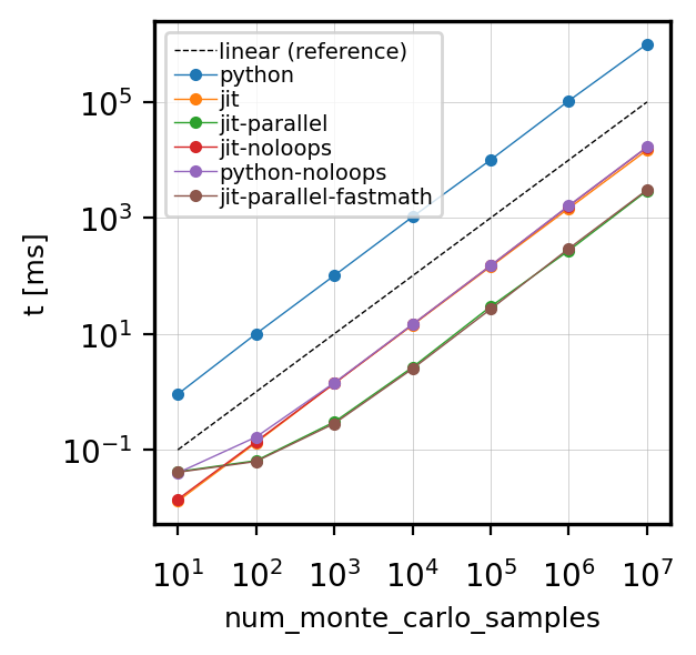
In this plot I present the scaling of the execution time (in milliseconds) as a function of num_monte_carlo_samples:
Comments:
- the scaling is pretty much linear (cf. reference dashed line) for all the implementations.
- the pure
pythonimplementation is, as expected, the least efficient. - by just adding a
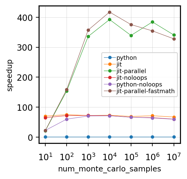
numba.jitdecorator (jitimplementation) to thepythonimplementation achieves a 75x speed-up, roughly in line with the speedup achieved by implementations with no explicit loops (jit-noloops). - using vectorized numpy functions with no explicit loops (
python-noloopsimplementation) achieves a very good acceleration as well (75x w.r.t.python), without the need ofnumba.jit. numba.jitwithparalleloption is further 5.7x faster than thejitversion. Overall, thejit-parallelversion is 390x faster than purepython.- enabling
fastmath, releasing the GIL (nogil=True), and explicitly declaring the function signature in the@njit()call does not produce a definite or substantial speedup over thejit-parallelimplementation.
The following plot shows the speedups over the python implementation:
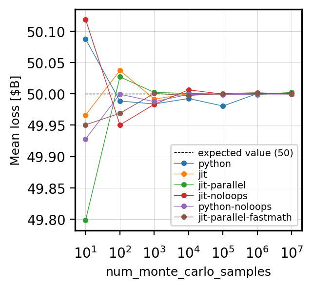
In the following figure I show the convergence of the mean economic losses for increasing num_monte_carlo_samples.
Comments:
- as expected, with increasing
num_monte_carlo_samples, all the implementations tend towards the same expected value (dashed line at mean loss=50 $B). - the pure
pythonimplementation is slightly slower in converging than the others.
The plots shown in this README are done in this Jupyter notebook.
oasishurricane is free software licensed under the BSD-3 License. For more details see the LICENSE.
© Copyright 2021 Marco Tazzari.


