- references
- Learning Spark, 2nd Edition
- Spark in Action, Second Edition
- https://medium.com/@mrpowers/testing-spark-applications-8c590d3215fa
- https://stackoverflow.com/questions/43729262/how-to-write-unit-tests-in-spark-2-0/50581218#50581218
- https://sparkbyexamples.com/spark/spark-read-and-write-json-file/
- https://sparkbyexamples.com/spark/spark-schema-explained-with-examples/
- https://sparkbyexamples.com/spark/spark-read-and-write-json-file/
- https://bigdataprogrammers.com/merging-two-dataframes-in-spark/
- https://mungingdata.com/apache-spark/aggregations/
- https://spark.apache.org/docs/3.0.0-preview/sql-getting-started.html#running-sql-queries-programmatically
- https://stackoverflow.com/a/43812193 (for windows)
- https://sparkbyexamples.com/spark/spark-sql-dataframe-join/
- https://towardsdatascience.com/write-clean-and-solid-scala-spark-jobs-28ac4395424a
- https://www.edureka.co/blog/spark-architecture/
- https://spark.apache.org/docs/latest/cluster-overview.html
- https://queirozf.com/entries/apache-spark-architecture-overview-clusters-jobs-stages-tasks
- https://data-flair.training/blogs/apache-spark-rdd-vs-dataframe-vs-dataset/
- https://medium.com/@venkat34.k/the-three-apache-spark-apis-rdds-vs-dataframes-and-datasets-4caf10e152d8
- https://towardsdatascience.com/strategies-of-spark-join-c0e7b4572bcf
- https://medium.com/datakaresolutions/optimize-spark-sql-joins-c81b4e3ed7da
- https://databricks.com/glossary/tungsten
- https://jaceklaskowski.gitbooks.io/mastering-spark-sql/content/spark-sql-tungsten.html
- https://www.dezyre.com/article/how-data-partitioning-in-spark-helps-achieve-more-parallelism/297
- https://luminousmen.com/post/spark-partitions
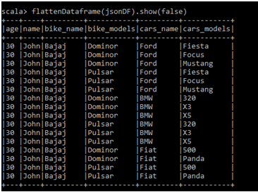
- https://www.24tutorials.com/spark/flatten-json-spark-dataframe/
- https://medium.com/@dvcanton/wide-and-narrow-dependencies-in-apache-spark-21acf2faf031
- https://towardsdatascience.com/best-practices-for-caching-in-spark-sql-b22fb0f02d34
- https://medium.com/@adrianchang/apache-spark-checkpointing-ebd2ec065371
- http://www.lifeisafile.com/Apache-Spark-Caching-Vs-Checkpointing/
- https://stackoverflow.com/questions/24696777/what-is-the-relationship-between-workers-worker-instances-and-executors
- https://www.tutorialkart.com/apache-spark/cluster-managers-supported-in-apache-spark/
- https://www.informit.com/articles/article.aspx?p=2928186
- goals of this workshop:
- introduction to spark and its architecture of spark
- peek under the hood: data representation and optimizations
- practicing rudimentary use-cases
- unified engine designed for large-scale distributed data processing
- provides in-memory storage for intermediate computations
- faster than Hadoop MapReduce
- libraries
- machine learning (MLlib)
- SQL for interactive queries (Spark SQL)
- stream processing (Structured Streaming) based on micro-batch processing engine
- graph processing (GraphX)
- typical Spark scenario
- Ingestion of raw data
- DQ: data quality
- example: ensure that all birth dates are in the past
- example: obfuscate Social Security numbers (SSNs)
- Transformation
- example: join with other datasets, perform aggregations
- Publication
- example: load the data into a data warehouse, save in a file on S3
- components and architecture

- SparkSession
- a single unified entry point to all of Spark’s functionality
- use cases
- defining DataFrames and Datasets
- reading from data sources
- writing to data lakes
- accessing catalog metadata
- issuing Spark SQL queries
- there is a unique SparkSession for your application, no matter how many nodes it runs
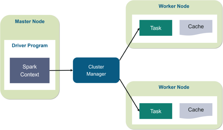
- Spark driver
- process running the
main()function of the application - instantiates SparkSession
- communicates with the cluster manager
- requests resources (CPU, memory, etc.) from the cluster manager for Spark’s executors (JVMs)
- plans and coordinates the execution: transforms operations into directed acyclic graph (DAG)
and schedules them
- keeps track of available resources to execute tasks
- schedules tasks to run "close" to the data where possible (data locality)
- distributes operations execution across the Spark executors
- once the resources are allocated, it communicates directly with the executors
- resides on master node
- process running the
- Spark master & Cluster manager
- Cluster Manager can be separate from the Master process
- Spark master requests resources and makes resources available to the Driver
- monitors the status and health of resources
- is not involved in the execution of the application and the coordination of its tasks and stages
- Cluster manager is a process responsible for monitoring the Worker nodes and reserving resources
on these nodes upon request by the Master
- Master then makes these cluster resources available to the Driver in the form of Executors
- Worker node
- any node that can run application code in the cluster
- may not share filesystems with one another
- Spark executor
- is a process that executes tasks on the workers often in parallel
- communicates with the driver program
- workers hold many executors, for many application
- Job
- is a sequence of Stages, triggered by an action (ex.
.count())
- is a sequence of Stages, triggered by an action (ex.
- Stage
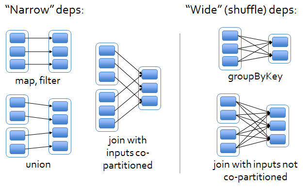
- a sequence of Tasks that can all be run in parallel without a shuffle
- example:
.read.map.filter
- Task
- unit of work that will be sent to one executor
- is a single operation (ex.
.mapor.filter) applied to a single Partition - is executed as a single thread in an Executor
- example: 2 Partitions, operation:
filter()=> 2 Tasks, one for each Partition
- Shuffle
- operation where data is re-partitioned across a cluster
- by having all the data needed to calculate on a single node, we reduce the overhead on the shuffle (the need for serialization and network traffic)
- costly operation - a lot of data travels via the network
- example: join
- operation where data is re-partitioned across a cluster
- Partition
- enable parallelization: data is split into Partitions so that each Executor can operate
on a single part
- once the user has submitted his job into the cluster, each partition is sent to a specific executor for further processing
- the more partitions the more work is distributed to executors, with a smaller number of partitions the work will be done in larger pieces
- every machine in a spark cluster contains one or more partitions
- single partition do not span multiple machines
- good starting point: number of partitions equal to the number of cores
- example
- 4 cores and 5 partitions
- processing of each partition takes 5 minutes
- total time: 10 minutes (4 in parallel in 5 minutes, then 1 in 5 minutes)
- example
- enable parallelization: data is split into Partitions so that each Executor can operate
on a single part
- deployment on Kubernetes
- Spark driver: Runs in a Kubernetes pod
- Spark executor: Each worker runs within its own pod
- Cluster manager: Kubernetes Master
- SparkSession
- RDD (Resilient Distributed Datasets)
- fundamental data structure of Spark
- immutable distributed collection of data
- data itself is in partitions
- Dataset and DataFrame
- take on two characteristics: DataFrame - untyped and Dataset - typed
- Dataset is a collection of strongly typed JVM objects
- has also an untyped view called a DataFrame, which is a Dataset of Row
- Row is a generic untyped JVM object that may hold different types of fields
- get first column of given row:
val name = row.getString(0)
- get first column of given row:
- Row is a generic untyped JVM object that may hold different types of fields
- has also an untyped view called a DataFrame, which is a Dataset of Row
- DataFrames are similar to distributed in-memory tables with named columns with types
(integer, string, array, map, etc), schemas
- no primary or foreign keys or indexes in Spark
- data can be nested, as in a JSON or XML document
- conversion: DataFrame -> Dataset
val bloggersDS = spark
  .read
  .json("path")
  .load()
  .as[TargetClass]
- schemas
- defines the column names and associated data types for a DataFrame
- inferring a schema (plus inferring data types)
- requires separate job to read a large portion of file to infer the schema
- can be expensive and time-consuming
- no errors detection if data doesn’t match the schema
- defining a schema
- programmatically:
val schema = StructType(Array(StructField("author", StringType, false) - DDL:
val schema = "author STRING, title STRING, pages INT"
- programmatically:
- typical use case: read from on-premise database and push to cloud storage (Amazon S3)
- data source types
- file (CSV, JSON, XML, Avro, Parquet, and ORC, etc)
- relational and nonrelational database
- other data provider: (REST) service, etc
- DataFrameReader
- core construct for reading data into a DataFrame
- supports many formats such as JSON, CSV, Parquet, Text, Avro, ORC, etc.
- DataFrameWriter
- it saves data to a data source
- after the files have been successfully exported, Spark will add a _SUCCESS file to the directory
- problem with traditional file formats
- big data files need to be splittable
- JSON and XML are not easy to split
- CSV cannot store hierarchical information (like JSON or XML)
- none designed to incorporate metadata
- quite heavy in size (especially JSON and XML)
- big data files need to be splittable
- big data formats: Avro, ORC, or Parquet
- Avro
- schema-based serialization format (binary data)
- supports dynamic modification of the schema
- row-based, so easier to split
- ORC
- columnar storage format
- supports compression
- Parquet
- columnar storage format
- supports compression
- add columns at the end of the schema
- Parquet metadata usually contains the schema
- if the DataFrame is written as Parquet, the schema is preserved as part of the Parquet metadata
- subsequent reads do not require you to supply a schema
- if the DataFrame is written as Parquet, the schema is preserved as part of the Parquet metadata
- default and preferred data source for Spark
- files are stored in a directory structure: data files, metadata, a number of compressed files, and some status files
- Avro
- operations can be classified into two types
- actions
- example:
count(),save() - triggers evaluation
- example:
- transformations
- actions
- DataFrame API
is equivalent to
Dataset<Row> apiDf = df .groupBy(col("firstName"), col("lastName"), col("state")) .agg( sum("quantity"), sum("revenue"), avg("revenue"));df.createOrReplaceTempView("orders"); String sqlStatement = "SELECT " + " firstName, " + " lastName, " + " state, " + " SUM(quantity), " + " SUM(revenue), " + " AVG(revenue) " + " FROM orders " + " GROUP BY firstName, lastName, state"; Dataset<Row> sqlDf = spark.sql(sqlStatement);
- Broadcast Hash Join (map-side-only join)
- used when joining small with large
- small = fitting in the driver’s and executor’s memory
- smaller data set is broadcasted by the driver to all Spark executors
- by default if the smaller data set is less than 10 MB
- does not involve any shuffle of the data set
- used when joining small with large
- Shuffle Sort Merge Join
- used when joining two large data sets
- default join algorithm
- pre-requirement: partitions have to be co-located
- all rows having the same value for the join key should be stored in the same partition
- otherwise, there will be shuffle operations to co-locate the data
- has two phases
- sort phase
- sorts each data set by its desired join key
- merge phase
- iterates over each key in the row from each data set and merges the rows if the two keys match
- sort phase
- tables
ids.write .option("path", "/tmp/five_ids") .saveAsTable("five_ids")- each table is associated with its relevant metadata (the schema, partitions, physical location
where the actual data resides, etc.)
- metadata is stored in a central metastore
- by default: Apache Hive metastore
- Catalog is the interface for managing a metastore
- spark.catalog.listDatabases()
- spark.catalog.listTables()
- spark.catalog.listColumns("us_delay_flights_tbl")
- location: /user/hive/warehouse
- Catalog is the interface for managing a metastore
- by default: Apache Hive metastore
- metadata is stored in a central metastore
- two types of tables
- managed
- Spark manages metadata and the data
- example: local filesystem, HDFS, Amazon S3
- note that SQL command such as DROP TABLE deletes both the metadata and the data
- with an unmanaged table, the same command will delete only the metadata
- unmanaged
- Spark only manages the metadata
- example: Cassandra
- managed
- each table is associated with its relevant metadata (the schema, partitions, physical location
where the actual data resides, etc.)
- views
- vs table: views don’t actually hold the data
- tables persist after application terminates, but views disappear
- to enable a table-like SQL usage in Spark - create a view
df.createOrReplaceTempView("geodata");

Dataset<Row> smallCountries = spark.sql("SELECT * FROM ...");
- vs table: views don’t actually hold the data
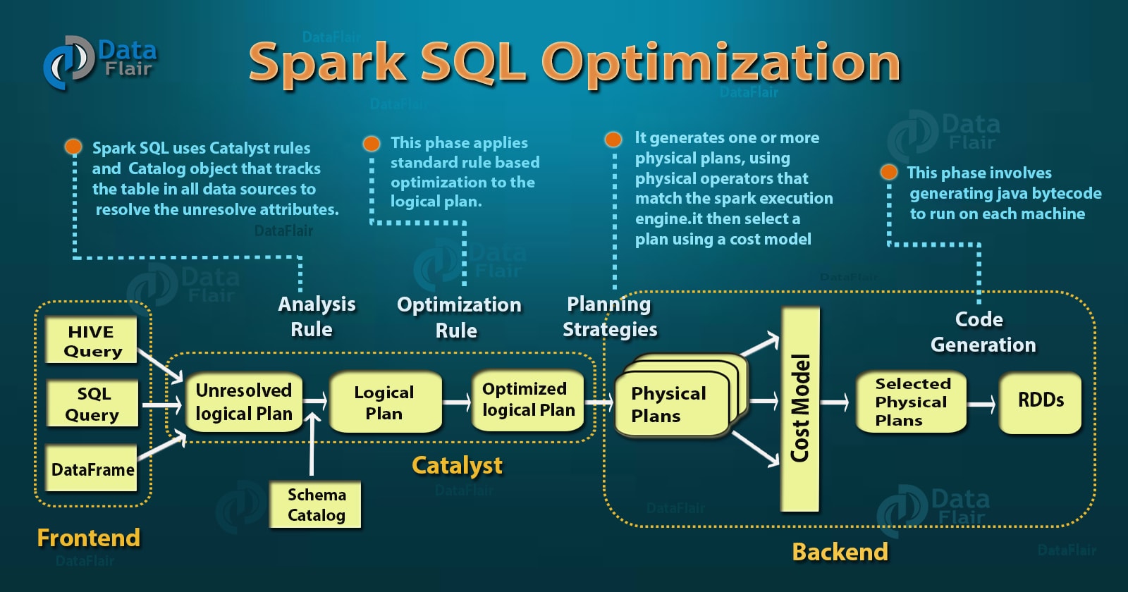
- at the core of the Spark SQL engine are the Catalyst optimizer and Project Tungsten
- note that a lot of the issues can come from key skewing: the data is so fragmented among partitions that a join operation becomes very long
- focuses on enhancing three key areas
- memory management and binary processing
- manage memory explicitly
- off-heap binary memory management
- eliminate the overhead of JVM object model and garbage collection
- Java objects have large overheads — header info, hashcode, Unicode info, etc.
- instead use binary in-memory data representation aka Tungsten row format
- manage memory explicitly
- cache-aware computation
- algorithms and data structures to exploit memory hierarchy (L1, L2, L3)
- cache-aware computations with cache-aware layout for high cache hit rates
- code generation
- exploit modern compilers and CPUs
- generates JVM bytecode to access Tungsten-managed memory structures that gives a very fast access
- uses the Janino compiler - super-small, super-fast Java compiler
- memory management and binary processing
- similar concept to RDBMS query optimizer
- converts computational query and converts it into an execution plan

- Phase 1: Analysis
- Spark SQL engine generates AST tree for the SQL or DataFrame query
- Phase 2: Logical optimization
- catalyst constructs a set of multiple plans and using its cost-based optimizer assign costs to each plan
- Phase 3: Physical planning
- Spark SQL generates an optimal physical plan for the selected logical plan
- Phase 4: Code generation
- generating efficient Java bytecode to run on each machine
- Spark maintains a history of all transformations you may apply to a DataFrame or RDD
- this enables Spark to be fault tolerant
- however Spark programs take a huge performance hit when fault occurs as the entire set of transformations to RDD have to be recomputed
- if you reuse a dataframe for different analyses, it is a good idea to cache it
- steps are executed each time you run an analytics pipeline
- example: DataFrames commonly used during iterative machine learning training
- caching vs persistence
- persist() provides more control over how and where data is stored
- DISK_ONLY, OFF_HEAP, etc.
- both are lazy transformations
- immediately after calling the function nothing happens with the data but the query plan is updated by the Cache Manager by adding a new operator — InMemoryRelation
- persist() provides more control over how and where data is stored
- caching vs checkpointing
- whatever is the case of failure, re-calculating the lost partitions is the most expensive operation
- best strategy is to start from some checkpoint in case of failure
- checkpoint() method will truncate the logical plan (DAG) and save the content of the dataframe to disk
- re-computations need not be done all the way from beginning, instead the checkpoint is used as the beginning of re-calculation
- cache will be cleaned when the session ends
- checkpoints will stay on disk
- example where checkpointing would be preferred over caching
- DataFrame of taxes for a previous year - they are unlikely to change once calculated so it would be much better to checkpoint and save them forever so that they can be consistently reused in the future
- whatever is the case of failure, re-calculating the lost partitions is the most expensive operation
val cubed = (s: Long) => { s * s * s } // define function

spark.udf.register("cubed", cubed) // register UDF

spark.sql("SELECT id, cubed(id) AS id_cubed FROM ...") // use
- excellent choice for performing data quality rules
- UDF’s internals are not visible to Catalyst
- UDF is treated as a black box for the optimizer
- Spark won’t be able to analyze the context where the UDF is called
- if you make dataframe API calls before or after, Catalyst can’t optimize the full transformation
- should be at the beginning or the end of transformations


