This Udacity Self-Driving Car Nanodegree project is to implement a deep learning program which detects German traffic signs. The steps of this project are the following:
- Load the data set (see below for links to the project data set)
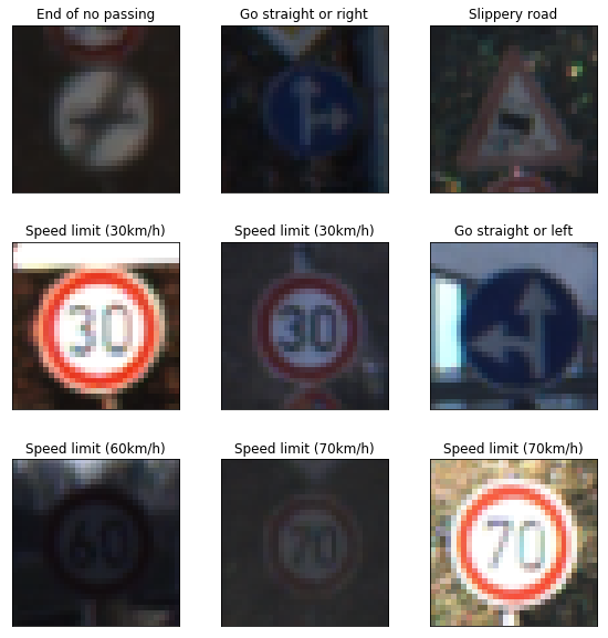
- Explore, summarize and visualize the data set
- Design, train and test a model architecture
- Use the model to make predictions on new images
- Analyze the softmax probabilities of the new images
- Summarize the results with a written report
Here is a link to my project code
I used the numpy library to calculate summary statistics of the traffic signs data set:
- The size of training set is 34,799.
- The size of the validation set is 4,410.
- The size of test set is 12,630.
- The shape of a traffic sign image is (32,32,3)
- The number of unique classes/labels in the data set is 43.
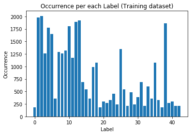
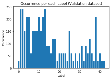
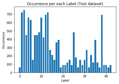
Here is an exploratory visualization of the data set. It is a bar chart showing how the datasets are distributed.
As seen in these bar charts, there are categories which have more images. This unbalanced dataset could affect the performance of the trained model. If so, it is needed to gather more traffic signs images to make them even. Another option is to augument traffic sign images.
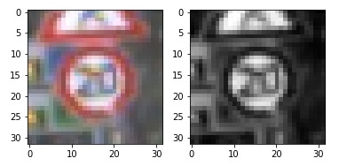
As a first step, I decided to convert the images to grayscale because the color of the signs do not contain meaningful information. Here is the code to convert images to grayscale.
X_train_gray = np.sum(X_train/3, axis=3, keepdims=True)Here is an example of a traffic sign image before and after grayscaling.
As a last step, I normalized the image data because large input values slows training and makes it difficult being optimized. Here is the code snippet for normalizing values, which makes the mean 0 and between -1 and 1.
X_train_gray_normal = (X_train_gray.astype(np.float32)-128)/128My final model consisted of the following layers:
| Layer | Description |
|---|---|
| Input | 32x32x3 RGB image |
| Convolution 5x5 | 6 filters, 1x1 stride, valid padding, outputs 28x28x6 |
| RELU | |
| Max pooling | 2x2 kernel, 2x2 stride, outputs 14x14x6 |
| Convolution 5x5 | 16 filters, 1x1 strides, valid padding, output 10x10x16 |
| RELU | |
| Max pooling | 2x2 kernel, 2x2 stride, outputs 5x5x16 |
| Fully connected | 120 neurons |
| RELU | |
| Dropout | 50% |
| Fully connected | 84 neurons |
| RELU | |
| Dropout | 50% |
| Fully connected | 43 neurons |
| Softmax | etc. |
This deep neural network architecture is similar to LeNet-5; 2 convolutional layers and 3 fully connected layers. Softmax is used to classification.
To train the model, I used an ....
- learning rate : 0.001
- number of epochs : 40
- dropout rate : 50%
- batch size : 128
- loss : cross entropy
- optimizaer : Adam
While I was finding an optimal hyper-parameter, I changed learning rate from 0.001 to 0.01 without awaring the change. The accuracy dropped to 4~5% while 0.001 gave 80% or higher accuracy. To me, it looks like a small amount of change, but actually its impact was a lot. That was a good learning point.
My final model results were:
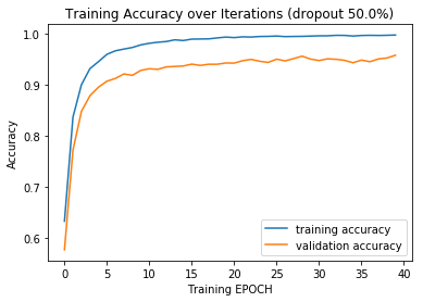
- training set accuracy of 0.998
- validation set accuracy of 0.959
- test set accuracy of 0.9417
This result has been achieved by doing iterative experiments. Here is the steps I went through to reach this.
First, I use LeNet-5 with traffic signs in RGB color. With this, the accuracy is below 0.93, but more importantly I had to deal with overfitting problem. To overcome the overfitting issue, I added drop into first two fully connected layers. I started with 10%, 20%, and 30%. With this architecture, 30% dropout rate fixed the overfitting issue.
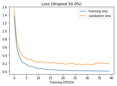
Second, I increased the number of epoches up to 40 by monitoring loss of training and validation dataset along with accuracy. I stopped at 40 because training accuracy is not improving at more.
Third, data preprocessing was needed to increase accuracy of training dataset and validation dataset. There are differnt ways of doing this; convering to grayscale, normalization, data augumentation, or gathering more data. I chose the first two methods because it is easy to implement for quick experiment. After appluing these two, the accuracy of training and validation dataset increased. Still, I observed overfitting. I increased dropout rate up to 50%, and I got the below result.
With a simple LeNet-5 deep neural network architecture, data preprocessing, and hyper-parameter tuning, I could get a well-trained model. LeNet-5 is known for a simple but yet good DNN architecutre for classifying handwritten digits. The traffic sign is a bit more complex than handwritten digits, but not too complex as images in ImageNet. Due to the nature of the image to be classified, LeNet-5 is a good choice for the given task.
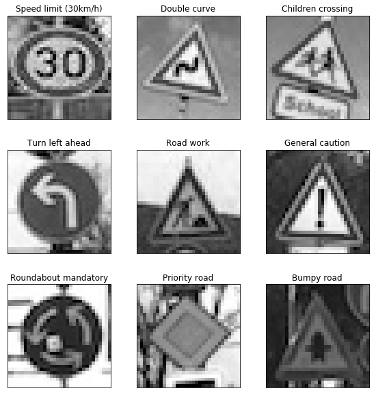
Here are 9 German traffic signs that I found on the web:
I need to resize them down to 32x32, which give poor quality. Also, the seventh image might be difficult to classify because there is a noise (white square) within the sign.
Here are the results of the prediction:
| Image | Prediction |
|---|---|
| 30 km/h | 50 km/h |
| Double curve | Slippey load |
| Children crossing | General Caution |
| Turn left ahead | Turn left ahead |
| Road Work | Road Work |
| General Caution | General Caution |
| Roundabout mandatory | Roundabout mandatory |
| Priority road | Priority road |
| Priority | Right of way at the next intersection |
The model was able to correctly guess 5 of the 9 traffic signs, which gives an accuracy of 55%. This compares favorably to the accuracy on the test set of 94%. It is not negligible gap, so it is required to analyze further to identify the root cause of this, and take an appropriate action such as data augmenting for further training.
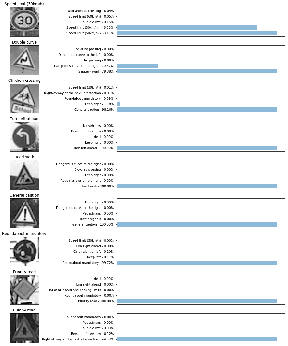
As one of investigation, let's take a look at the top5 softmax probabilities for each image.
Out of these 4 falsely predicted signs, the first one (30 km/h) has high probability for 30 km/h after 50 km/h. Also, I just found that the 9th sign is not belong to any of 43 signs in the project.
DNN is sometimes known as black-box. However, we can get the idea what it is doing by taking a look at outout of feature maps in the hidden layers. Below are output of feature maps after 1st and 2nd convolutional layer.
Expectation is to have simple pattern detected in the 1st convolutional layer and then complex pattern in the 2nd layer. But in this case, it is not that straighforward and I guess it is due to the small size of input image (32x32)

