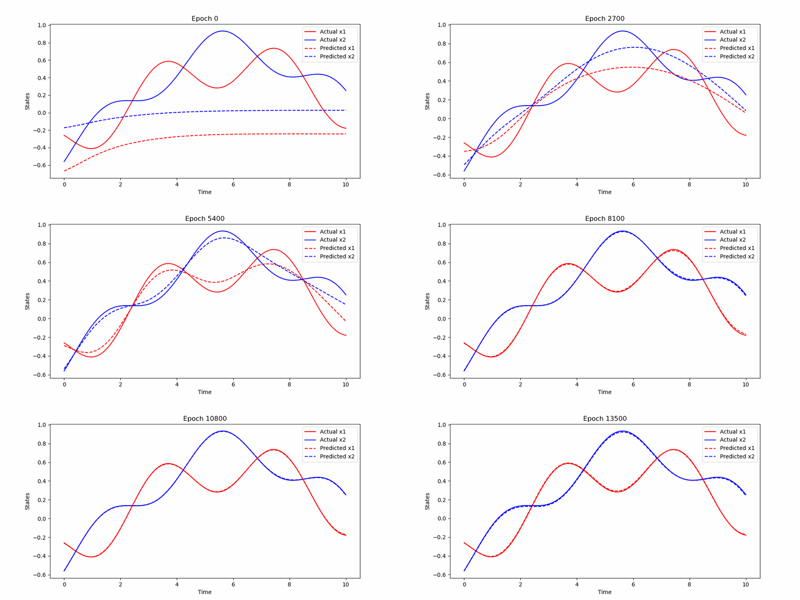
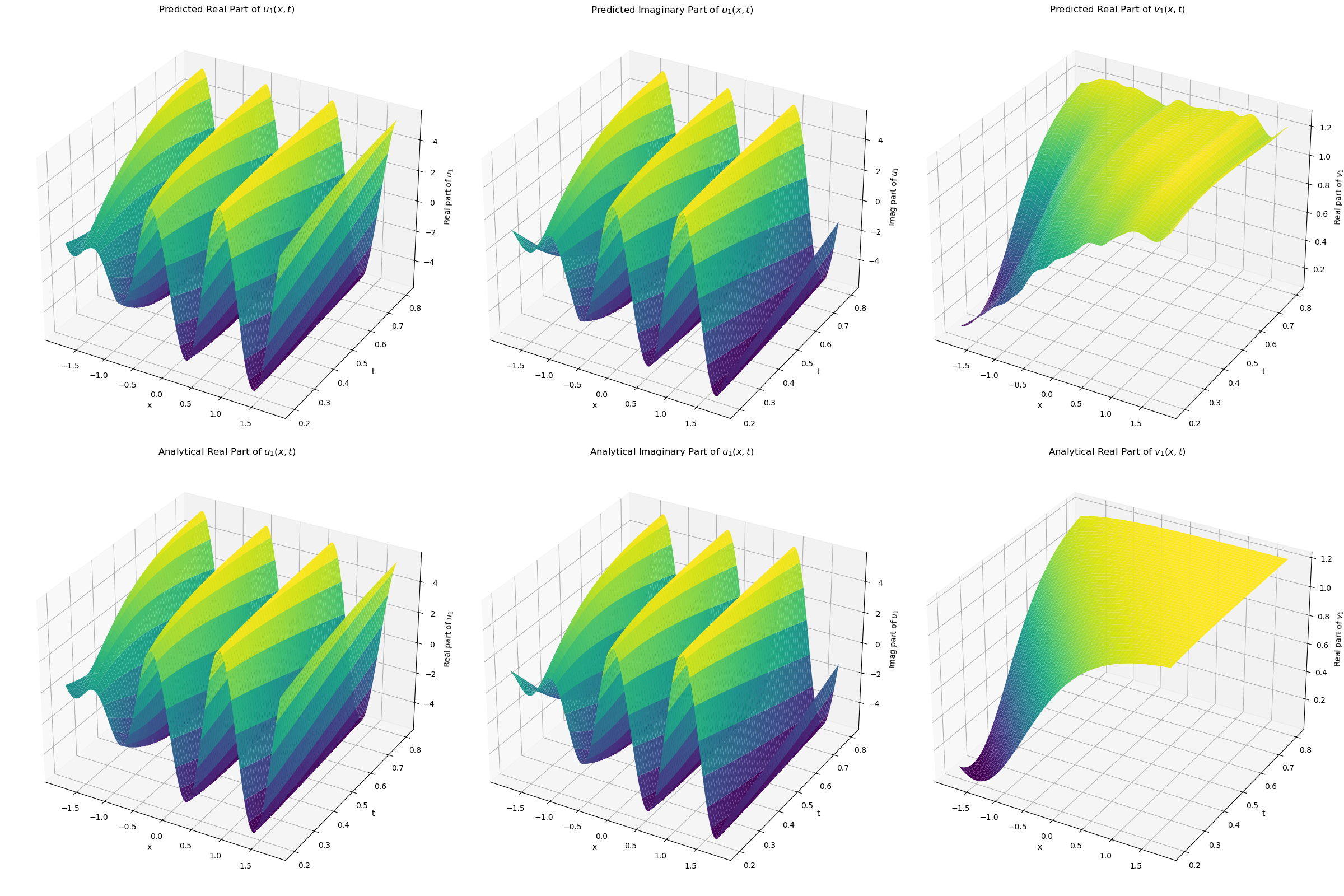
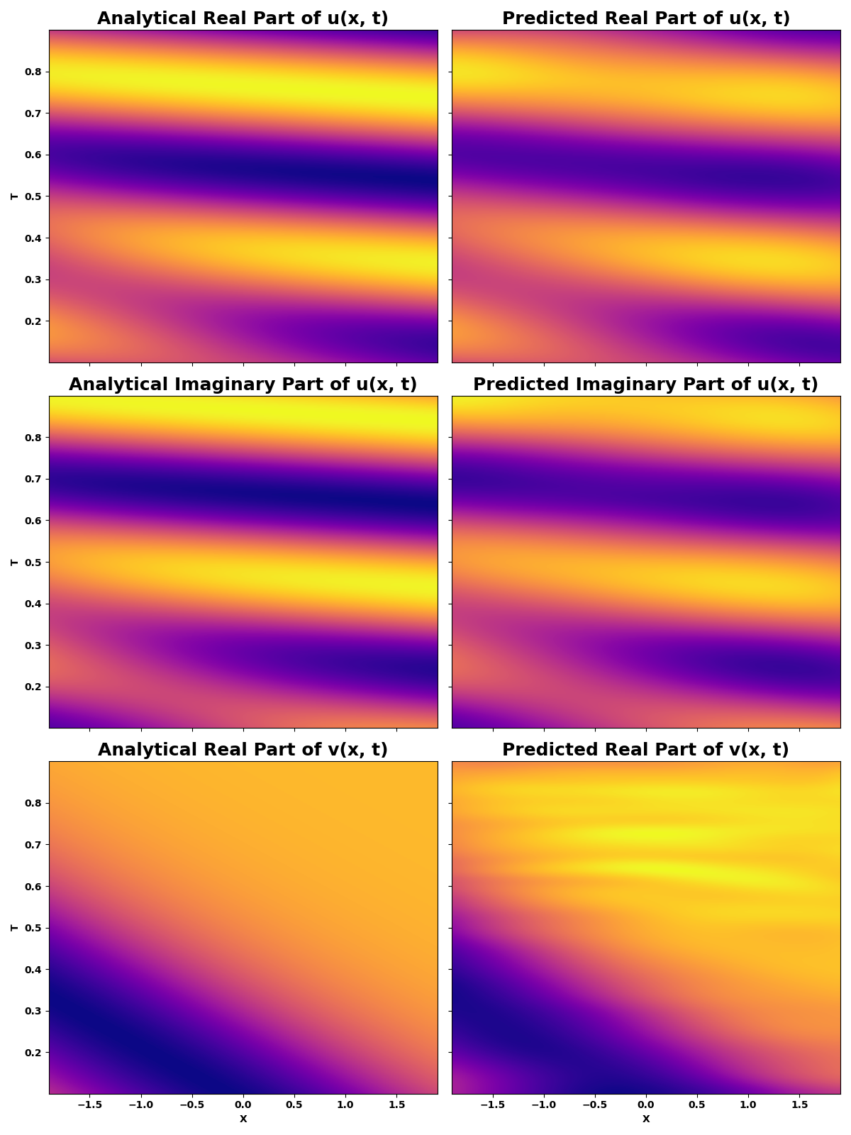
This repository contains implementations of Physics-Informed Neural Networks (PINNs) to solve various physical systems described by partial differential equations (PDEs) or ordinary differential equations (ODEs). PINNs leverage the power of deep learning to approximate solutions to complex physical and quantum mechanical problems by incorporating physical laws as part of their loss function.
- 1D Harmonic Oscillator
- 1D Quantum Harmonic Oscillator
- 2-D PDE Example
- Symmetric Infinite Potential Well
- Non-linear Schrödinger Equation
- Coupled Spring system
- Lotka-Voltera Equation
- Coupled Higgs Equation
- Installation
- Acknowledgments
The 1D damped harmonic oscillator is described by the differential equation:
with initial conditions
Original code inspired by benmoseley.
Solves the quantum harmonic oscillator problem, given by the Hamiltonian:
and the corresponding Schrödinger equation. The solution involves the eigenfunctions
A simple 2-D PDE problem:
with boundary condition
Original code by nanditadoloi.
Solves the time-dependent Schrödinger equation for a particle in a symmetric infinite potential well, focusing on the solutions within the well and the quantized energy levels.
Addresses the non-linear Schrödinger equation with periodic boundary conditions, showcasing the use of PINNs in solving complex, non-linear PDEs.
Here we try to solve the spring that has the lagrangian
The Lotka-Volterra equations, also known as the predator-prey model, are represented as a system of first-order nonlinear differential equations:
where
-
$x$ represents the prey population, -
$y$ represents the predator population, -
$\alpha$ is the natural growth rate of prey in the absence of predators, -
$\beta$ is the natural dying rate of prey due to predation, -
$\delta$ is the efficiency of converting consumed prey into predator population, and -
$\gamma$ is the natural dying rate of predators in the absence of prey.
The constants are normalized for this demonstration with
where,
solutions
where
For nixpkgs users use the following
git clone https://github.com/mushrafi88/Physics-Informed-Neural-Networks-for-Quantum-Dynamics.git
cd Physics-Informed-Neural-Networks-for-Quantum-Dynamics
NIXPKGS_ALLOW_UNFREE=1 nix develop --impure- Original PINN methodology by Raissi et al.
- Example implementations inspired by contributions from benmoseley and nanditadoloi.


