Build a Traffic Sign Recognition Project
The goals / steps of this project are the following:
- Load the data set (see below for links to the project data set)
- Explore, summarize and visualize the data set
- pre-processing the images
- Extending data samples
- Data normalisation
- Design, train and test a model architecture
- Improve model accuracy through test different hyperparameters
- Use the model to make predictions on new images
- Analyze the softmax probabilities of the new images
- Summarize the results with a written report
---
I used the numpy library to calculate summary statistics of the traffic signs data set:
- The size of training set is 34799
- The size of the validation set is 4410
- The size of test set is 12630
- The shape of a traffic sign image is (32, 32, 3)
- The number of unique classes/labels in the data set is 43
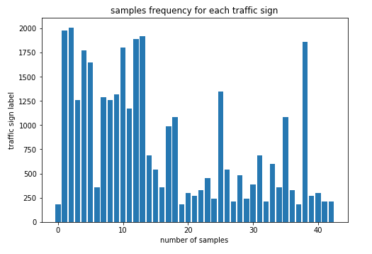
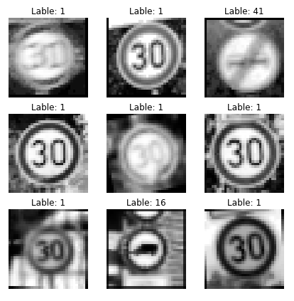
Here is an exploratory visualization of the data set. It is a bar chart showing how the data is distributed for different traffic signs. You see the disparity and how unbalance the data set is. for some lables there is just so few number of samples that it makes learning process unreliable.
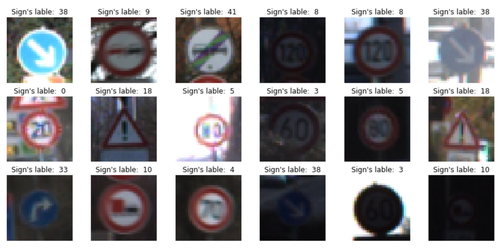
As a first step, I decided to convert the images to YUV to have both the color and grayscale property of an image, however after some trial and error for experiencing different network architecture I realized that the grayscale image gives us alone the best result as it has been reported in Yann LeCun report[1].
Here is an example of some traffic sign images before and after grayscaling.
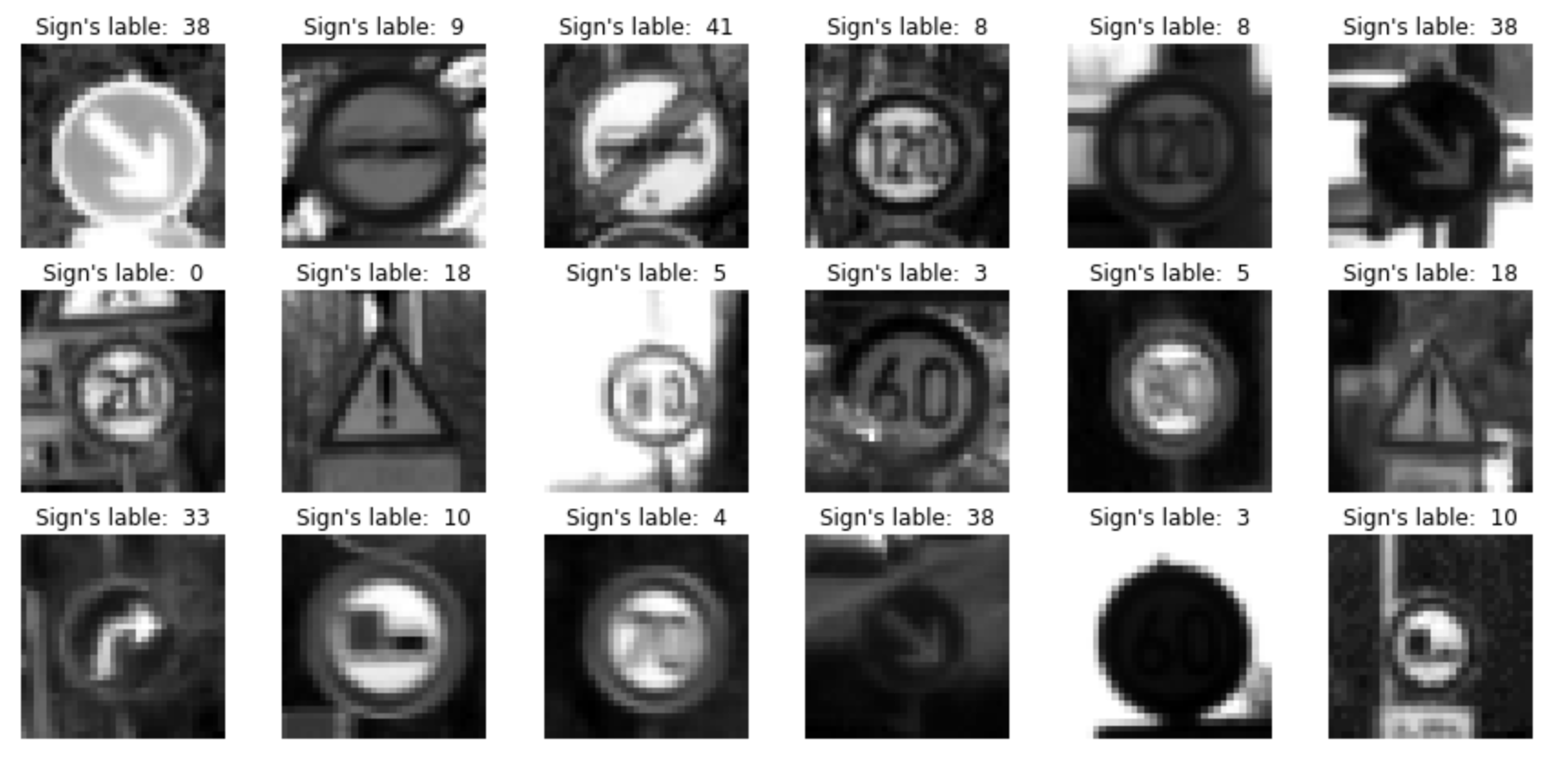
After that a histogram equalization has been performed on images to prevent light intencity and shadows affect on samples. With this technique we made our data set more balance. In this way the nerual network react more relible for defferent images. You also can think about that with different lighting and contrast conditions there are unwanted and unrelated features to learn that are irrelevant to determine the sign category. There is no useful information in contrast or lighting of an image about what sign is in the image! In below you see images after histogram equalization.
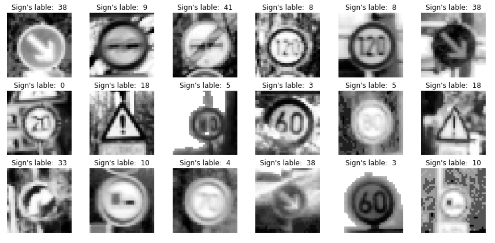
As a last step, I normalized the image data because it makes data set more easy to learn by nerual network. There is a same logic behind of this preprocessing as histogram equalization that mentioned above. In below you see the result of normalization for some random samples.
I decided to generate additional data because for some of sign categories there were far less samples in data set and in addition the data set was unbalanced. To add more data to the the data set, I used the following techniques.
- Scale between 0.9 and 1.1, because because the size of sign can be different depending on how far the sign can be located. The distance from object in 3D world means the size of the object in image!
- rotate between -15 and 15 degrees, Because in real world signs are not likely to be with the same rotation always.
- translation between -2 and 2 pixel in both direction independently. It makes our nerual network more indipendent of were the sign is located.
Here is an example of an original image and an augmented image: (from left to right respectively, orginal image, scaled image, rotated image, translated image)
In result of this process our training set has been raised to 139196 images!
2. Describe what your final model architecture looks like including model type, layers, layer sizes, connectivity, etc.) Consider including a diagram and/or table describing the final model.
My final model consisted of the following layers:
| Layer | Description |
|---|---|
| Input | 32x32x1 grayscale image |
| Convolution 5x5 | 1x1 stride, valid padding, outputs 28x28x100 |
| RELU(conv1) | 1 copy will use as input of fully connected |
| Max pooling(branch) | 2x2 stride, outputs 14x14x100 |
| Convolution 5x5 | 1x1 stride, valid padding, outputs 10x10x200 |
| RELU(conv2) | |
| Max pooling(conv2) | 2x2 stride, outputs 5x5x200 |
| Max pooling(branch) | 2x2 stride, outputs 7x7x100 |
| Dropout | 90% keep rate |
| Fully connected | 9900 feature, 100 nodes |
| Fully connected | 100 feature, 43 nodes, logits |
| softmax cross entropy | softmax between logits and layers |
| cost function | reduce_mean of softmax cross entropy function |
| Optimizer | AdamOptimizer |
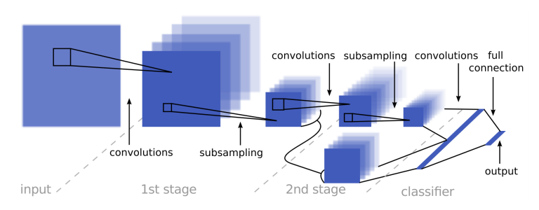
You see the visualized network architecture in below, I used the same network architecture as [1] after many trial and error. I got the best result with same network as it reported in [1].
3. Describe how you trained your model. The discussion can include the type of optimizer, the batch size, number of epochs and any hyperparameters such as learning rate.
To train the model, I used an AdamOptimizer with learning rate of 0.0009 and 20 Epochs in total. I choosed 128 as my batch size during training process. Also the cost function that I choose is reduce_mean of softmax cross entropy between logits and one-hot labeles.
4. Describe the approach taken for finding a solution and getting the validation set accuracy to be at least 0.93. Include in the discussion the results on the training, validation and test sets and where in the code these were calculated. Your approach may have been an iterative process, in which case, outline the steps you took to get to the final solution and why you chose those steps. Perhaps your solution involved an already well known implementation or architecture. In this case, discuss why you think the architecture is suitable for the current problem.
At the first I tried to use LeNet-5 base solution that considering the complexity of traffic sign project I had optimized it. It contained far more filters and nodes in every stage comparing to LeNet-5 model. The logic behine it was that in comparison with numbers between 0 to 9, there is much more features that should be extract from image in every stage. It can be color of different part of sign, the shape and image inside it.
I choose 106 filters for first stage and 200 for second stage, 6 of first stage filters were acting only on u and v channels of color image in yuv color space and the rest, 100 filters, on grayscale channel. For detecting more complex shapes I decide to increase the number of filters in second stage so the combination of two first stage could detect complex shapes and colors.
I couldn't get any better result than 93% using that model using all 3 channel of yuv color space as input. After changing the input to one channel grayscale image I got better result up to 95% on validation data set. Finaly I used the reported model in [1] and saw I getting far more better result, more than 98% accuracy on validation set.
I set a dropout befor full connected layer to prevent over fitting. With keep rate of 0.5 The results showed the network is under fitted. With trial and error I choosed 0.9 for keeping rate ad it results to 99.793% accuracy for train data set and 98.05% for validation that means the model is well fitted.
As I experienced using small number of batches results better accuracy, maybe it's because that in every epoch the program calls optimizer more and it makes the model more trained and fitted. I set batches size to 128 after trying 256, 512, 1024 and 2048.
My final model results were:
- training set accuracy of 99.79%
- validation set accuracy of 98.05
- test set accuracy of 96.03%
1. Choose five German traffic signs found on the web and provide them in the report. For each image, discuss what quality or qualities might be difficult to classify.
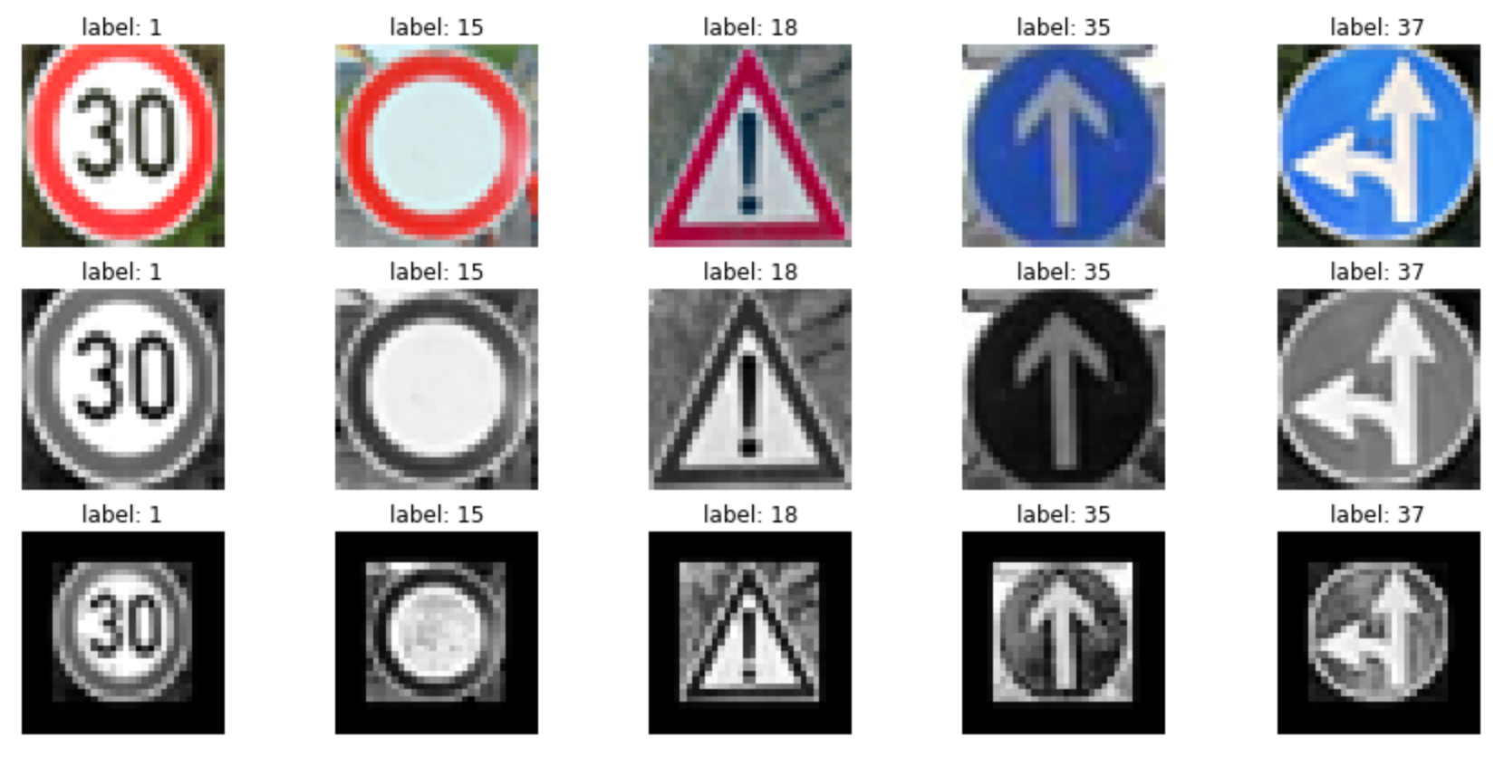
Here are five German traffic signs that I found on the web:
In 2nd row you see the preprocessed images as we did on our dataset for test and train part. in 3rd row you see scaled images with 0.7 scale factor, because the images that I found shows bigger signs, so whole the frame contain the sign. In case to using them without scaling the accuracy will drop to 20% as I tried it. It
The first image might be difficult to classify because ...
2. Discuss the model's predictions on these new traffic signs and compare the results to predicting on the test set. At a minimum, discuss what the predictions were, the accuracy on these new predictions, and compare the accuracy to the accuracy on the test set (OPTIONAL: Discuss the results in more detail as described in the "Stand Out Suggestions" part of the rubric).
Here are the results of the prediction:
| Image | Prediction |
|---|---|
| Speed limit (30km/h) | Speed limit (30km/h) |
| No vehicles | Road work |
| General caution | General caution |
| Ahead only | Ahead only |
| Go straight or left | Speed limit (50km/h) |
The model was able to correctly guess 3 of the 5 traffic signs, which gives an accuracy of 60%. In some trainings I got even 100% accuracy on new images, or 80% too.
3. Describe how certain the model is when predicting on each of the five new images by looking at the softmax probabilities for each prediction. Provide the top 5 softmax probabilities for each image along with the sign type of each probability. (OPTIONAL: as described in the "Stand Out Suggestions" part of the rubric, visualizations can also be provided such as bar charts)
The code for making predictions on my final model is located in the 11th cell of the Ipython notebook. The top five probabilities are:
[[ 1., 0., 0., 0., 0.], [ 1., 0., 0., 0., 0.], [ 1., 0., 0., 0., 0.], [ 1., 0., 0., 0., 0.], [ 1., 0., 0., 0., 0.]]
That shows the model has picked the results with probability of close to 100%
[1] Pierre Sermanet and Yann LeCun, Traffic Sign Recognition with Multi-Scale Convolutional Networks. In here
