- Stationary means the distribution of the data doesn't change with time.
- For time series to be stationary it must fulfill three criterias
- Trend stationary (Zero trend) : The series has zero trend, it isn't growing or shrinking.
- The variance is constant : The average distance of the data points from the zero line isn't changing
- The Autocorrelation is constant : How each value in the time series is related to its neighbors stays the same.
- There are also Statistical tests for stationarity
- We can also convert a non stationary dataset to stationary.
- The most common test to identify whether a time-series is non-stationary is augmented Dicky-Fuller test
This is a statistical test with the null hypothesis : Time Series is non stationary due to trend
from statsmodels.tsa.stattools import adfuller

results = adfuller(df['close'])- The results object is a tuple. The zeroth element is the test statistics. In this case its (-1.34). The more negative this number is, its more likely that the data is stationary.
- 1st element is p-value : (0.60) If the p-value is <0.05, we reject the null hypothesis and assume that our time-series must be stationary.
- The last item in the results object is the dictionary, this stores the critical values of the test statistics which equates the different p-values.
- In this case if we wanted a p-value of 0.05 or below, our test statistics needed to be below -2.913
- It's always worth plotting your time series as well as doing statistical tests.
- These tests are useful, but sometimes they dont capture the full picture.
- Dicky-fuller only tests for trend stationarity.
- Plotting time series can stop you from making wrong assumptions.
- Suppose a time series is non stationary and we need to transform the data into stationary time series before we can model it.
- We can think of it as feature engineering in Classic Machine Learning.
- A very common way to make a time series stationary is to take its difference.
Differece : ^yt = yt - yt-1df_stationary = df.diff().dropna()
Examples of other transforms
-
Take the log : np.log(df)
-
Take the sqaure root : np.sqrt(df)
-
Take the proportional change: df.shift(1)/df
-
Differencing should be the first transform you try to make a time series stationary. But sometimes it is'nt the best option. A classic way of transforming stock time series is the log-return of the series. This is calculated as follows:
log_return(yt) = log(yt / yt-1)
In AR models we regress the values of the time-series against previous values of the same time series.
AR(1) model : This is the first order AR model, the order of the model is the number of time lags used.
yt = a1*yt-1 + et
a1 = Autoregressive coefficent at lag 1.
et = white noise (each shock is random & not related to other shocks in the series)
- Compare this to simple linear regression, where yt is the dependent varaible and yt-1 is the independent varaible. Coefficient a1 is just the slope of the line, and the shocks are the residuals of the line.
`yt = a1y(t-1) + a2y(t-2) + et
`yt = a1y(t-1) + a2y(t-2) + ... + ap*y(t-p) + et
In moving average model, we regress the values of the time series against the previous shock values of the same time series.
- MA(1) model:
yt = m1 * e(t-1) + et - MA(2) model: `yt = m1 * e(t-1) + m2 * e(t-2) + et
- MA(q) model: `yt = m1 * e(t-1) + m2 * e(t-2) + .... + mq * e(t-q) + et
-
ARMA = AR + MA . ARMA is the combination of the AR and MA models.
-
The time series is regressed against previous values and the previous shock terms.
-
ARMA(1,1) model:
yt = a1 * y(t-1) + m1 * e(t-1) + et -
ARMA(p,q)
-
p is the order of AR part
-
q is the order of MA part
- Using the statsmodel package model, we can both fit ARMA model and generate ARMA data.
- When fitting and working with AR, MA and ARMA models it is very important to understand the model order. You will need to pick the model order when fitting. Picking this correctly will give you a better fitting model which makes better predictions.
- Creating a model
from statsmodels.tsa.arima_model import ARMA
model = ARMA(timeseries, order=(p, q))- Fitting an AR model
ar_model = ARMA(timeseries, order=(p, 0))- Fitting an MA model
ma_model = ARMA(timeseries, order=(0, q))model = ARMA(timeseries, order=(2,1))
results = model.fit()
print(results.summary())- The
std_errcolumn in summary tells the uncertainity in the fitted coef values
- One modification to ARMA models is to use Exogenous inputs to create the ARMAX models.
- This means, we model the time series using other independent variables as well.
- This is like a combination between ARMA model and normal Linear Regression model.
- ARMAX = ARMA + Linear Regression
- ARMA(1,1) model : yt= a1 * y(t-1) + m1 * e(t-1) + et
- ARMAX(1,1) model : yt = x1 * zt + a1 * y(t-1) + m1 * e(t-1) + et
- Only difference is one additonal term zt and it's coef x1
- This can be an ARMA model as productivity on previous day may have affect on productivity today, you could be overworked or on a row.
- A useful Exogenous variable could be the amount of sleep you have got the night before, since this might affect your productivity.
- Here
z1would be the hours slept. - And if more sleep makes you productive, coef x1 will be positive.
We can fit an ARMAX model using the same ARMA model class, the only difference is we now feed in the exogenous variable using the exog keyword
model = ARMA(df['productivity'], order=(2,1), exog=df(['hours_sleep']))Predicting the next value
- Take AR(1) model : At any point in the time series we can make predictions using the formula
yt = a1 * y(t-1) + et - Predict next value yt = 0.6 * 10 + et yt = 6.0 + et
- If the shock term has std-deviation of 1, we would predict the uncertainty limit on prediction as:
5.0 < yt < 7.0
- We can do lot of predictions in-sample using the previous series value to estimate the next one, this is called one-step-ahead predictions.This allows us to evaluate how good our model is in predicting a value one step ahead.
- Uncertainity is due to the random shock terms that we can't predict.
from statsmodels.tsa.statespace.sarimax import SARIMAX

# just an ARMA(p, q) model
model = SARIMAX(df, order=(p, 0, q))- A SARIMAX model with order(p, 0, q) is same as ARMA(p, q). We can also add a constant to a model using
trend = 'c'. If a time-series is'nt centered around zero, this is a must.
# An ARMA(p, q) + constant model
model = SARIMAX(df, order=(p, 0, q), trend = 'c')# make prediction for last 25 values
results = model.fit()
# make in-sample prediction
forecast = results.get_prediction(start=-25)- We can use
get_predictionmethod to make insample predictions.start = -25tells how many steps back to begin the forecast.start=-25means make predictions for last 25 entries of the training data. - The centre value of the forecast is stored in
predicted_meanattribute of the forecast object. This predicted mean is a pandas series
# forecast mean
mean_forecast = forecast.predicted_mean- To get the lower and the upper limits on the values of our prediction we use the
conf_intmethod of the forecast object
# get confidence intervals of forecast
confidence_intervals = forecast.conf_int()- We can use pyplot plot method to plot the mean values
- We use pyplot
fill_betweento shade the area between lower and upper limits.
plt.figure()

# plot prediction
plt.plot(dates, mean_forecast.values, color='red', label='forecast')

# shade uncertainty area
plt.fill_between(dates, lower_limits, upper_limits, color='pink')
plt.show()We can make dynamic predictions then just one step ahead.
results = model.fit()
forecast = results.get_prediction(start=-25, dynamic=True)- Finally after testing our predictions in sample, we can use our model to predict the future.
- To get future forecast we use the
get_forecastmethod. We use thestepsparameter with number of steps after end of the training data to forecast upto.
forecast = results.get_forecast(steps=20)- We have learnt that we cannot apply ARMA model to non-stationary data, we need to take the difference of the time-series to make it stationary only then we can model it.
- However, when we do this (difference) then we will have a model that will predict difference of the time series. What we really want to predict is not the difference but the actual value of the time-series.
- We can acheive this by carefully transforming our prediction of the differences.
- The opposite of taking the difference is taking the sum or integral.
- We will have to use this transform to go from prediction of differenced values to prediction of absolute values.
- We can do this transform using the
np.cumsumfunction.
diff_forecast = results.get_forecast(steps=10).predicted_mean
from numpy import cumsum
mean_forecast = cumsum(diff_forecast) + df.iloc[-1, 0]-
After applying this transform we now have a prediction of how much a time-series changed from its initial value over the forecast peroid.
-
To get the absolute value we need to add the last value of the original time series to it. We now have a forecast of the non stationary time-series.
-
Take the difference
-
Fit ARIMA model
-
Integrate forecast
-
Can we avoid doing so much work ? Yes!
- We can implement ARIMA using the SARIMAX model class from statsmodel
from statsmodels.tsa.statespace.sarimax import SARIMAX
model = SARIMAX(df, order = (p,d,q))- The ARIMA model has 3 model orders
- p - number of autoregressive lags
- d - order of differencing
- q - number of moving average lags
- In ARMA model we were setting the order d to zero. In ARIMA we pass non - differenced time-series and the model order.
model = SARIMAX(df, order=(2, 1, 1))- Here we difference the time series data just once and then apply an ARMA (2, 1) model
- After we have stated the difference parameter we dont need to worry about differencing anymore.
- The differencing and integration steps are all taken care off by the model object.
# Fit model
model.fit()

# Make forecast
mean_forecast = results.get_forecast(steps=steps).predicted_mean- We should be careful in selecting the correct amount of differencing. We difference the data only till its stationary and no more.
- We will decide the differening order using the Augmented Dicky Fuller test
- We know to fit ARIMA models. But how do we know which ARIMA model to fit. The model order is very important.
- One correct way to find the order of the model is to use ACF - Autocorrelation function and the PACF - Partial autocorrelation function
- The autocorrelation function at lag-1 is the correlation between the timeseries and same time series offset by one step. lag-1 autocorrelation -> corr(yt, y(t-1))
- The autocorrelation at lag-2 is the correlation between the timeseries and same time series offset by two steps.
- We can plot the autocorrelation function to get the overview of the data.
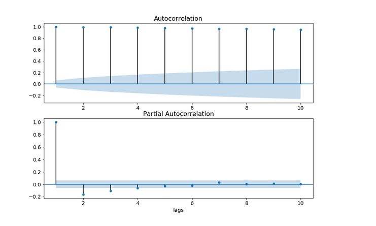
- Bars shows that ACF values are increasing lags.If the bars are small and lie in the blue shade region, then they are not statisctically significant.
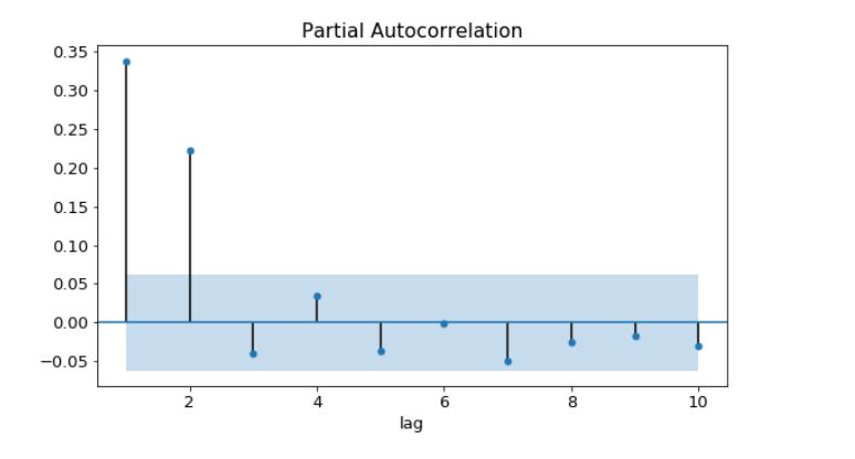
- Partial autocorrelation is the corelation between a time series and the lagged version of itself after we subtract the correlation at smaller lags.So it's the correlation associated with just that particular lag.
- PACF is these series of values.
- By comparing the ACF and PACF for time-series we can deduce the model order.If the amplitude of the ACF tails off with increasing lag and the PACF cuts off after some lag p, then we have an AR(p) model
- Below plot is an AR(2) model
- If the amplitutde of ACF cuts off after some lag q and the amplitude of PACF tails off then we have a MA(q) model
- Below is an MA(2) model
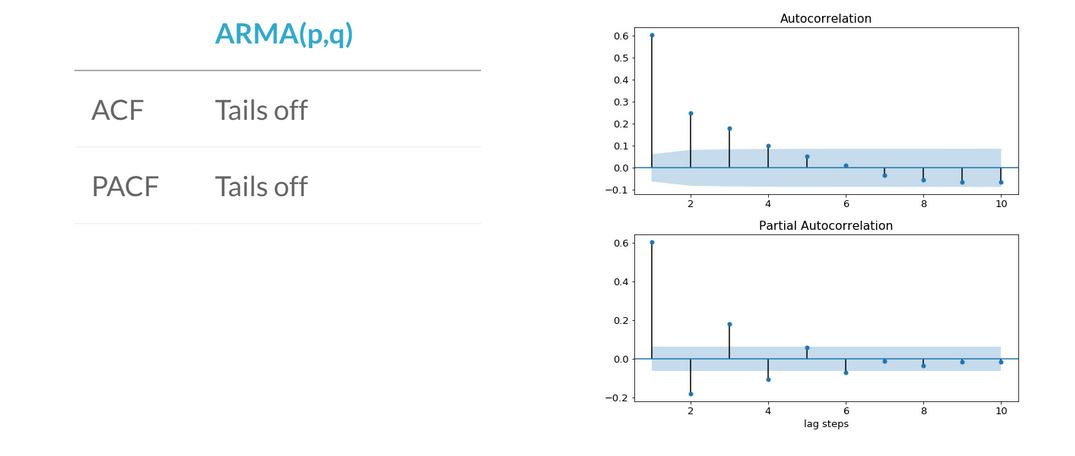
- If both the ACF and PACF tails off then we have an ARMA model. In this case, we can't deduce the model orders p & q from the plot.
- Refer following table when analyzing ACF and PACF
from statsmodels.graphics.tsaplots import plot_acf, plot_pacf

# create figure
fig, (ax1, ax2) = plt.subplots(2, 1, figsize=(8,8))

# make acf plot
# in each plot we pass the time-series dataframe and the max no of lags we would like to see. We also tell if we want to show autocorrelation at lag 0
# the ACF and PACF at lag=0 always has a value of 1, so we set it to False
plot_acf(df, lags=10, zero=False, ax=ax1)

# make pacf plot
plot_pacf(df, lags=10, zero=False, ax=ax2)
plt.show()- The time-series must be made stationary before making this plot
- If the ACF value is high and tail off very slowly, this is the sign that the data is non-stationary.So it needs to be differenced.
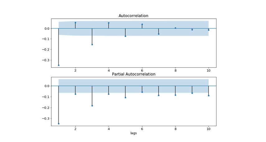
- If the autocorrelation at lag-1 is very negative, this is the sign that we have taken the difference too many times.
- ACF, PACF can't be used to choose the order of the model, when both of the orders p & q are non zero. However, there are more tools we can use, the AIC & BIC
- The AIC is a metric which tells us how good a model is. A model which makes better predictions is given a lower AIC score . The AIC also penalizes models which have lots of parameters.
- This means if we set the order too high compared to the data, we will get a high AIC value. This stops us overfitting to the training data.
- The Bayesian information criterion, or BIC, is very similar to the AIC. Models which fit the data better have lower BICs and the BIC penalizes over complex models.
- For both of these metrics a lower value suggests a better model.
- The difference between these two metrics is how much they penalize model complexity.
- The BIC penalizes additional model orders more than AIC and so the BIC will sometimes suggest a simpler model.
- The AIC & BIC will often choose the same model, but when they don't we have to make a choice.
- If our goal is to identify good predictive models , we should use AIC .However if our goal is to identify good explanatory model , we should use BIC.
- After fitting a model, we can find the AIC, BIC by using the
summaryof the fitted model results object.
# create model
model = SARIMAX(df, order=(1, 0, 1))

# fit model
results = model.fit()

# print fit summary
print(results.summary())

# OR print AIC, BIC
print('AIC:', results.aic)
print('BIC:', results.bic)- Being able to access the AIC and BIC directly means we can write loops to fit multiple ARIMA models to a dataset , to find the best model order .
- Here we loop over AR and MA orders between zero and two, and fit each model.
- if we want to test large number of model orders, we can append the model order and the AIC and BIC to a list, and later convert it to a dataframe.
- This means we can sort by the AIC score and not have to search through each record.
# loop over AR order

order_aic_bic = []
for p in range(3):
    # loop over MA order
    for q in range(3):
        # fit model
        model = SARIMAX(df, order=(p, 0, q))
        results = model.fit()

        # print the model order and the AIC/BIC values
        print(p, q, results.aic, results.bic)

        # add the model and scores to list
        order_aic_bic.append((p, q, results.aic, results.bic))

# make dataframe of model order and AIC/BIC scores
order_df = pd.DataFrame(order_aic_bic, columns=['p', 'q', 'aic', 'bic'])

# sort by AIC
print(order_df.sort_values('aic'))

# sort by BIC
print(order_df.sort_values('bic'))- Sometimes when searching over the model orders we will attempt to fit an order that leads to an error.
ValueError: Non-stationary starting autoregressive parameters found with enforce_stationarity set to True. This ValueError tells us that we have tried to fit a model which would result in a non-stationary set of AR coefficients.- This is just a bad model for this data, and when we loop over p and q we would like to skip this one. We can skip these orders using try, except.
for p in range(3):
    for q in range(3):
        try:
            model = SARIMAX(df, order=(p, 0, q))
            results = model.fit()

            print(p, q, results.aic, results.bic)
        except:
print(p, q, None, None)- Model diagnostics to check whether model is behaving well. After we have picked a final model, we should check how good they are. This is the key part of the model building life cycle.
- To diagnose our model we focus on the residuals to the training data.
- The residuals are the difference between the our model's one step ahead predictions and the real values of the time series.
- In statsmodels the residuals over the training period can be accessed using the
.residattribute of the results object. These are stored as a pandas series.
model = SARIMAX(df, order=(p, d, q))
results = model.fit()

# assign residuals to variable
residuals = results.resid- We might want to know on an average how large the residuals are and so how far our predictions are from the true values.
- To answer this we can calculate the mean absolute error of the residuals
mae = np.mean(np.abs(residuals))- For ideal model the residuals should be uncorrelated white Gaussian noise centered on zero. The rest of the diagnostics will help us to see if this is true.
- If the model fits well the residuals will be white Gaussian noise.
# create the 4 diagnostics plots
results.plot_diagnostics()
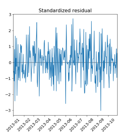
plt.show()- Standardized residual plot : One of the four plots shows the one-step-ahead standardized residuals. If our model is working correctly, there should be no obvious structure in the residuals.
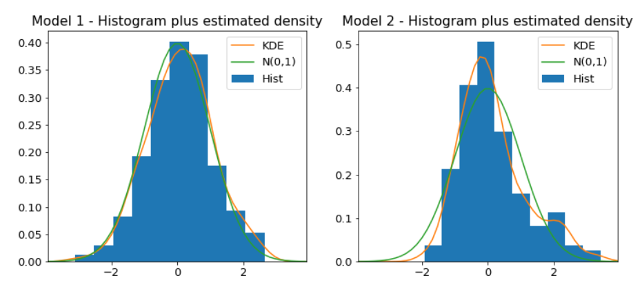
- Histogram plus estimated density : Shows us the distribution of the residuals. The histogram shows us the measured distribution; the orange line shows a smoothed version of this histogram; and the green line shows a normal distribution.
- If our model is good these two lines should be almost the same.
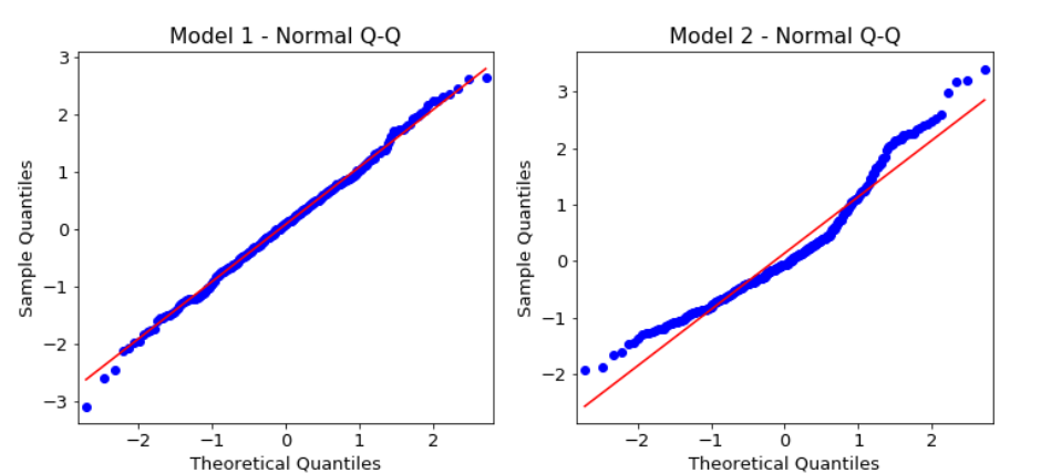
- The normal Q-Q plot is another way to show how the distribution of the model residuals compares to a normal distribution. If our residuals are normally distributed then all the points should lie around the red line, except perhaps some values at either end.
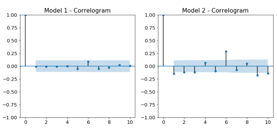
- ACF plot of the residuals rather than the data.
- 95% of the correlations for lag greater than zero should not be significant. If there is significant correlation in the residuals, it means that there is information in the data that our model hasn't captured .
- Some of these plots also have accompanying test statistics in
results.summary()
print(results.summary())- Prob(Q) - is the p-value associated with the null hypothesis that the residuals have no correlation structure.
- Prob(JB) - is the p-value associated with the null hypothesis that the residuals are Guassian normally distributed.
- If either p-value is less than 0.05 we reject that hypothesis.
- Building time series models can represent a lot of work for the modeler and so we want to maximize our ability to carry out these projects fast, efficiently and rigorously. This is where the Box-Jenkins method comes in.
- Box-Jenkins method is a kind of checklist for us to go from raw data to a model ready for production.
- The 3 main steps that stand between us and production-ready model are identification, estimation and model diagnostics .
- In the identification step we explore and characterize the data to find some form of it which is appropriate to ARIMA modeling.
- We need to know whether the time series is stationary and find which transformations such as differencing or taking the log of the data, will make it stationary.
- Once we have found a stationary form, we must identify which orders p and q are the most promising.
- Our tools to test for stationarity include plotting the time series and using the augmented Dicky-Fuller test.
df.plot(),adfuller() - Then we can take the difference or apply transformations until we find the simplest set of transformations that make the time series stationary.
df.diff(), np.log(), np.sqrt() - Finally, we use the ACF and PACF to identify promising model orders.
plot_acf() , plot_pacf()
- The next step is estimation, which involves using numerical methods to estimate the AR and MA coefficients of the data.
- This is automatically done for us when we call the
model.fit()method - At this stage we might fit many models and use the AIC and BIC to narrow down to more promosing candidates.
results.aic , results.bic
- In the model diagnostics step, we evaluate the quality of the best fitting model.
- Here is where we use our test statistics and diagnostics plots to make sure the residuals are well behaved.
- Are the residuals uncorrelated
- Are residuals normally distributed
results.plot_diagnostics(),results.summary()
- Using the information gathered from statistical tests and plots during the diagnostics step, we need to make a decision. Is the model good enough or do we need to go back and rework it.
- If the residuals aren't as they should be we will go back and rethink our choices in the earlier steps. If the residuals are okay then we can go ahead and make forecasts.
results.get_forecast()
- This should be our general project workflow when developing time series models.
- We may have to repeat the process a few times in order to build a model that fits well.
- A seasonal time series has predictable patterns that repeat regularly. Although, we call this feature seasonality, it can repeat after any length of time.
- These seasonal cycles might repeat every year like sales of suncream, or every week like number of visitors to a park, or everyday like number of users on a website at any hour.
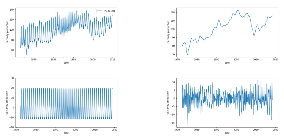
- Below is monthly US candy production, which has a regular cycle that repeats every year. We can think of this, or any time series, as being made of 3 parts. The trend, the seasonal component, and the residual .
- The full time series is these 3 parts added together.
time series = trend + seasonal + residual
- We can use statsmodels
seasonal_decomposefunction to separate out any time series into these three components. We have to set the period parameter which is number of data points in each repeated cycle. Here our cycle repeats every 12 steps. This function returns a decompose results object. - We can use the plot method of this object to plot the components.
- Inorder to decompose the data, we need to know how often the cycles repeat. Often we will be able to guess this, but we can also use the ACF to identify the period.
from statsmodels.tsa.seasonal import seasonal_decompose

# decompose data
decomp_results = seasonal_decompose(df['IPG3113N'], period=12)

# plot the decomposed data
decomp_results.plot()
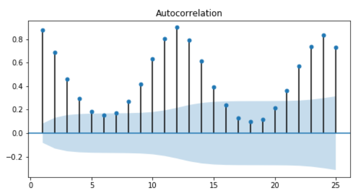
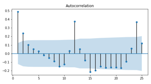
plt.show()- The above ACF shows a periodic correlation pattern. To find the period we look for a lag greater than one, which is a peak in the ACF plot.
- Here, there is a peak at 12 lags and so this means that the seasonal components repeats every 12 time steps.
- Sometimes it can be hard to tell by eye whether a time series is seasonal or not. This is where the ACF is useful.
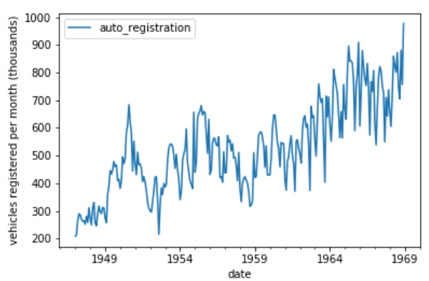
- Above is the monthly number of vehicles registered in the US. We could take this time series and plot the ACF directly, but since the time series is non-stationary, the ACF plot will be clearer if we detrend it first.
- We have detrended time series before by taking the difference. However, this time we are only trying to find the period of the time series, and the ACF plot will be clearer if we just subtract the rolling mean. Any large window size N will work for this.
- We subtract this from the original time series and drop the NA values. The time series is now stationary and it will be easier to interpret the ACF plot.
# subtract long rolling average over N steps

df = df - df.rolling(N).mean()

# create figure
fig, ax = plt.subplots(1, 1, figsize=(8,4))

# plot ACF
plot_acf(df.drop(), ax=ax, lags=25, zero=False)
plt.show()- We plot the ACF of the detrended data and we can clearly see that there is a seasonal period of 12 steps.
- Since the data is seasonal we will always have correlated residuals left if we try to fit and ARIMA model to it. This means we aren't using all the information in the data, and so we aren't making the bsest predictions possible.
- A SARIMA or seasonal arima models is used for seasonal time series.
- Fitting a SARIMA model is like fitting two different ARIMA models at once, one to the seasonal part and another to the non-seasonal part.
SARIMA(p, d, q)(P, D, Q)s - Since we have these two models we will have two sets of orders. We have non-seasonal orders for the autoregressive, difference and moving average parts.
- Non-seasonal orders :
p: autoregressive order ; d: differencing order ; q: moving average order - Seasonal Orders :
P : seasonal autoregressive order ; D: seasonal differencing order ; Q : seasonal moving average order ; S: number of time steps per cycle - There is also a new order
S, which is the length of the seasonal cycle.
- ARIMA(2,0,1) :
y = a1*y(t-1) + a2 * y(t-2) + m1 e(t-1) + et. We regress the time series against itself at lags-1 and 2 against the shock at lag-1. - SARIMA(0, 0, 0)(2, 0, 1) model:
yt =a7 * y(t-7) + a14 * y(t -14) + m7 * e(t-7) + et. This is the equation for a simple SARIMA model with season length of 7 days. This SARIMA model only has a seasonal part; we have set the non-seasonal orders to zero. - We regress the time series against itself at lags of one season and two seasons and against the shock at lag of one season.
- This particular SARIMA model will be able to capture seasonal weekly patterns, but wont be able to capture local, day to day patterns.
- If we construct a SARIMA model and include non-seasonal orders as well, then we can capture both of these patterns.
- Fitting a SARIMA model is almost the same as fitting an ARIMA model. We import the model object and fit it.
- The only difference is that we have to specify the seasonal order as well as the regular order when we instantiate the model. This means that there are a lot of model orders we need to find.
- The seasonal period S is found using the ACF.
from statsmodels.tsa.statespace.sarimax import SARIMAX

# instantiate model
model = SARIMAX(df, order=(p, d, q), seasonal_order=(P,D,Q,S))

# fit model
results = model.fit()- The next task is to find the order of differencing. To make a time series stationary we may need to apply seasonal differencing.
- In seasonal differencing, instead of subtracting the most recent time series value, we subtract the time series value from one cycle ago .
delta yt = yt - y(t-s) - We can take the seasonal difference by using the
.diff()method. This time we pass in an integer S, the length of the seasonal cycle.
# take the seasonal difference

df_diff = df.diff(S)- If the time series shows a trend then we take the normal difference .If there is a strong seasonal cycle, then we will also take the seasonal difference .
- Once we have found the two orders of differencing, and made the time series stationary, we need to find the other model orders. To find the non-seasonal orders , we plot the ACF and the PACF of the differenced time series .
- To find the seasonal orders we plot the ACF and PACF of the differenced time series at multiple seasonal steps. Then we can use the table of ACF and PACF rules to work out the seasonal order.
- This plots ACF and PACF at the specific lags only.
fig, (ax1, ax2) = plt.subplots(2,1)

# plot seasonal ACF
plot_acf(df_diff, lags=[12,24,36,48,60,72], ax=ax1)

# plot seasonal PACF
plot_pacf(df_diff, lags=[12,24,36,48,60,72], ax=ax2)

plt.show()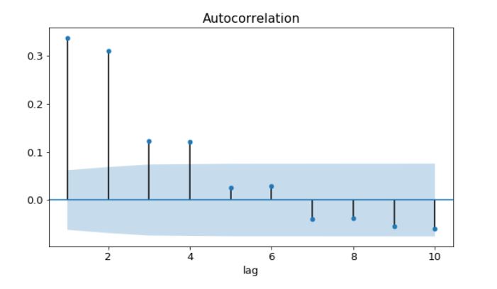
.JPG)
.JPG)
.JPG)
