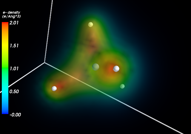
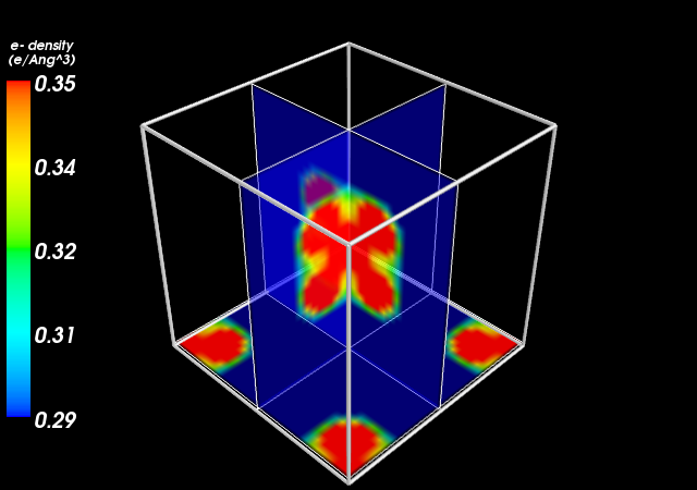
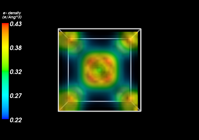
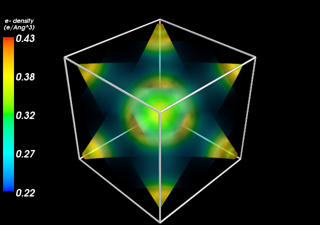
The objective of this project is to use data generated by ASE/JASP/VASP to produce 3D electron density plots. I have made a small module which contains a couple of functions that do this. As inputs, it takes calculation data generated by VASP (using JASP). The Mayavi “pipeline” is used to generate “advanced” 3D plots which display the charge density and optionally the atom locations and a bounding box representing the unit cell. You can also control some of the basics of the plot appearence in order to get a good-looking result.
ChgPlot.ChargeDensityFog3D(directory,
                           save_loc=None,
                           DrawAtoms=True,
                           DrawCell=True,
                           opacity_range=[0,1])
| Argument | Description |
|---|---|
| directory | Directory in which the VASP calculation files are located |
| save_loc | Location where image of the figure should be saved. Saving can also be done through the Mayavi window. |
| DrawAtoms | Represent atoms as small spheres in the plot if True (default = True) |
| DrawCell | Draw the unit cell surrounding the molecules if True (default = True) |
| opacity_range | Controls the transparency of the “fog” (default = [0,1]) |
The default values for the opacity_range makes the maximum electron density opaque and the minimum completely transparent. This seems to give good looking results, but it may be necessary to adjust the values to get the desired appearence. The first element of the list gives the transparency at the minimum electron density and the second element gives the transparency at the maximum.
ChgPlot.ChargeDensitySlice3D(directory,
                             save_file=None,
                             x_loc=None,
                             y_loc=None,
                             z_loc=None,
                             DrawAtoms=True,
                             DrawCell=True)
| Argument | Description |
|---|---|
| directory | Directory in which the VASP calculation files are located |
| save_loc | Location where image of the figure should be saved. Saving can also be done through the Mayavi window. |
| x_loc | Location where the x-oriented slice should be placed (given in Angstroms) |
| y_loc | Location where the y-oriented slice should be placed (given in Angstroms) |
| z_loc | Location where the z-oriented slice should be placed (given in Angstroms) |
| DrawAtoms | Represent atoms as small spheres in the plot if True (default = True) |
| DrawCell | Draw the unit cell surrounding the molecules if True (default = True) |
If x_loc, y_loc, or z_loc are not specified, they will not be drawn. For example, only specifying y_loc will cause only the y-oriented plane to appear in the figure.
The python module is located in the file ChgPlot.py. The source code is also given below.
from jasp import *
from enthought.mayavi import mlab
from ase.data.molecules import molecule
from ase.data import vdw_radii
from ase.data.colors import cpk_colors
import numpy as np

def ChargeDensityFog3D(directory, save_file=None , DrawAtoms=True, DrawCell=True, opacity_range=[0,1]):
    # Get data from calculation files
    with jasp(directory) as calc:
        atoms = calc.get_atoms()
        x, y, z, cd = calc.get_charge_density()

    mlab.figure(bgcolor=(0,0,0), size=(640,480))

    # Draw atoms
    if DrawAtoms == True:
        for atom in atoms:
            mlab.points3d(atom.x,
                          atom.y,
                          atom.z,
                          scale_factor=vdw_radii[atom.number]/10.,
                          resolution=16,
                          color=tuple(cpk_colors[atom.number]),
                          scale_mode='none')
    # Draw unit cell
    if DrawCell == True:
        a1, a2, a3 = atoms.get_cell()
        origin = [0,0,0]
        cell_matrix = [[origin, a1],
                       [origin, a2],
                       [origin, a3],
                       [a1, a1+a2],
                       [a1, a1+a3],
                       [a2, a2+a1],
                       [a2, a2+a3],
                       [a3, a1+a3],
                       [a3, a2+a3],
                       [a1+a2, a1+a2+a3],
                       [a2+a3, a1+a2+a3],
                       [a1+a3, a1+a3+a2]] # contains all points on the box
        for p1, p2 in cell_matrix:
            mlab.plot3d([p1[0], p2[0]], # x-coords of box
                        [p1[1], p2[1]], # y-coords
                        [p1[2], p2[2]]) # z-coords

    # Plot the charge density
    src = mlab.pipeline.scalar_field(x, y, z, cd) #Source data
    vmin = cd.min() #find minimum and maximum value of CD data
    vmax = cd.max()
    vol = mlab.pipeline.volume(src) # Make a volumetric representation of the data

    # Set opacity transfer function
    from tvtk.util.ctf import PiecewiseFunction
    otf = PiecewiseFunction()
    otf.add_point(vmin, opacity_range[0]) #Transparency at zero electron density
    otf.add_point(vmax*1, opacity_range[1]) #Transparency at max electron density
    vol._otf=otf
    vol._volume_property.set_scalar_opacity(otf)

    #Show a legend
    mlab.colorbar(title="e- density\n(e/Ang^3)", orientation="vertical", nb_labels=5, label_fmt='%.2f')
    mlab.view(azimuth=-90, elevation=90, distance='auto') # Set viewing angle
    mlab.show()
    if save_file != None:
        mlab.savefig(save_file)

def ChargeDensitySlice3D(directory, save_file=None, x_loc=None, y_loc=None, z_loc=None, DrawAtoms=True, DrawCell=True):
    # Get data from calculation files
    with jasp(directory) as calc:
        atoms = calc.get_atoms()
        x, y, z, cd = calc.get_charge_density()

    mlab.figure(bgcolor=(0,0,0), size=(640,480))

    # Draw atoms
    if DrawAtoms == True:
        for atom in atoms:
            mlab.points3d(atom.x,
                          atom.y,
                          atom.z,
                          scale_factor=vdw_radii[atom.number]/10.,
                          resolution=16,
                          color=tuple(cpk_colors[atom.number]),
                          scale_mode='none')
    # Draw unit cell
    if DrawCell == True:
        a1, a2, a3 = atoms.get_cell()
        origin = [0,0,0]
        cell_matrix = [[origin, a1],
                       [origin, a2],
                       [origin, a3],
                       [a1, a1+a2],
                       [a1, a1+a3],
                       [a2, a2+a1],
                       [a2, a2+a3],
                       [a3, a1+a3],
                       [a3, a2+a3],
                       [a1+a2, a1+a2+a3],
                       [a2+a3, a1+a2+a3],
                       [a1+a3, a1+a3+a2]] # contains all points on the box
        for p1, p2 in cell_matrix:
            mlab.plot3d([p1[0], p2[0]], # x-coords of box
                        [p1[1], p2[1]], # y-coords
                        [p1[2], p2[2]]) # z-coords

    # Plot the charge density on three perpendicular planes at the center of the cell
    src = mlab.pipeline.scalar_field(x, y, z, cd) #Source data
    vmin = cd.min() #find minimum and maximum value of CD data
    vmax = cd.max()
    if x_loc != None:
        sliceX = mlab.pipeline.image_plane_widget(src,
                                                  plane_orientation = 'x_axes',
                                                  slice_index = x_loc * 10,
                                                  transparent = True)
    if y_loc != None:
        sliceY = mlab.pipeline.image_plane_widget(src,
                                                  plane_orientation = 'y_axes',
                                                  slice_index = y_loc * 10,
                                                  transparent = True)
    if z_loc != None:
        sliceZ = mlab.pipeline.image_plane_widget(src,
                                                  plane_orientation = 'z_axes',
                                                  slice_index = z_loc * 10,
                                                  transparent = True)
    #Show a legend
    mlab.colorbar(title="e- density\n(e/Ang^3)", orientation="vertical", nb_labels=5, label_fmt='%.2f')
    mlab.show()
    if save_file != None:
mlab.savefig(save_file)In this example, a simple relaxation calculation is performed on a methane molecule and then the electron density is plotted as a fog.
from jasp import *

from ase.data.molecules import molecule

NH3 = molecule("NH3")
NH3.set_cell([8,8,8], scale_atoms=False)
NH3.center()

CH4 = molecule("CH4")
CH4.set_cell([8,8,8], scale_atoms=False)
CH4.center()

ready = True
with jasp('example-calcs/CH4',
          xc = 'PBE',
          encut = 350,
          ismear = 0,
          sigma = 0.01,
          ibrion = 1,
          nsw = 50,
          ediffg = -0.05,
          atoms = CH4) as calc:
    try:
       calc.calculate()
       CH4 = calc.get_atoms()
    except (VaspSubmitted, VaspQueued):
       ready = False
       print "Jobs submitted/queued"

with jasp('example-calcs/NH3',
          xc = 'PBE',
          encut = 350,
          ismear = 0,
          sigma = 0.01,
          ibrion = 1,
          nsw = 50,
          ediffg = -0.05,
          atoms = NH3) as calc:
    try:
       calc.calculate()
       NH3 = calc.get_atoms()
    except (VaspSubmitted, VaspQueued):
       ready = False
       print "Jobs submitted/queued"

if not ready:
    import sys; sys.exit()

from ChgPlot import ChargeDensityFog3D

ChargeDensityFog3D("example-calcs/NH3")
ChargeDensityFog3D("example-calcs/CH4", opacity_range=[0, 0.75])Here, electron density is plotted as “slices” and as a fog. In this particular case, the volume rendering that Mayavi uses shows some weird artifacts at angles away from the x, y, and z axes. However, the plane slices give a pretty nice result and are a bit more informative.
from jasp import *
JASPRC['queue.walltime'] = '24:00:00' #Zhongnan's hax
from ase.lattice.cubic import BodyCenteredCubic

atoms = BodyCenteredCubic("Ta")

ready=True
with jasp("example-calcs/TaBCC",
          xc="PBE",
          encut=350,
          kpts=(8,8,8),
          atoms=atoms) as calc:
    try:
            calc.calculate()
            atoms = calc.get_atoms()
    except (VaspSubmitted, VaspQueued):
            ready=False

if not ready:
    import sys; sys.exit()

from ChgPlot import ChargeDensitySlice3D, ChargeDensityFog3D
ChargeDensitySlice3D("example-calcs/TaBCC", x_loc=3.3/2, y_loc=3.3/2, z_loc=0)For simple molecules, rendering the electron density as a fog certainly produces a cool visual effect. However, it can sometimes be difficult to get useful information out of this kind of plot. This is mainly because the outer layers of “fog” can sometimes obscure the inner layers behind them. In the above examples, the transparency of the fog is scaled with the value of the electron density (i.e., the minimum electron desity is completely transparent while the maximum density is mostly opaque). It is possible to modify the color and opacity scaling by changing the “color transfer function” and “opacity transfer function”. A linear opacity transfer function was used in this example, but any “shape” can be given to this function. The same goes for the color transfer function. In this example, the hue is changed continuously with electron density. However, it is possible to use any combination of different colors.
Rendering a fog also seems to produce some strange artifacts in some cases. For example, viewing the Tantalum BCC unit cell in-line with the x-axis gives a result that looks reasonable (fig. 4), but viewing from an angle gives a strange result (fig. 5). In these kinds of cases, it is much more useful to plot electron density through plane slices instead as shown in the second example above. It may not be as fancy, but it avoids this problem as well as problems with the data obscuring itself. With highly symetric systems, one plane may be all that is necessary to visualize all of the data fully.
- J. Kitchin, “DFT-book”, p. 41-44.
- Ramachandran, P. and Varoquaux, G., “Mayavi: 3D Visualization of Scientific Data” IEEE Computing in Science & Engineering, 13 (2), pp. 40-51 (2011)
- Enthought Mayavi Documentation: http://docs.enthought.com/mayavi/mayavi/mlab.html#visualizing-volumetric-scalar-data


