ndag/persistence-curv-sets

Curvature sets over persistence diagrams

This repository contains the implementation of some of the ideas in our paper https://arxiv.org/pdf/2103.04470.pdf.

The implementation below is via Matlab's parfor.

The software was developed by Mario Gomez and Facundo Memoli. We also use functions written by Misha Belkin (L2_distance.m), Vin de Silva (px_fps.m), Uli Bauer (Ripser: https://github.com/Ripser/ripser), Masoud Alipur (emd_mex.m), and Michael Kerber, Dmitriy Morozov & Arnur Nigmetov (bottleneck distance with Hera). We have also benefited from Chris Tralie's Matlab wrapper for Ripser (https://github.com/ctralie/Math412S2017).

Installation Instructions:

1. This code was developed in Matlab version R2019a. It requires the Parallel Computing Toolbox (https://www.mathworks.com/products/parallel-computing.html).
2. From a terminal go to the ripser folder and run make ripser-coeff.

Main script

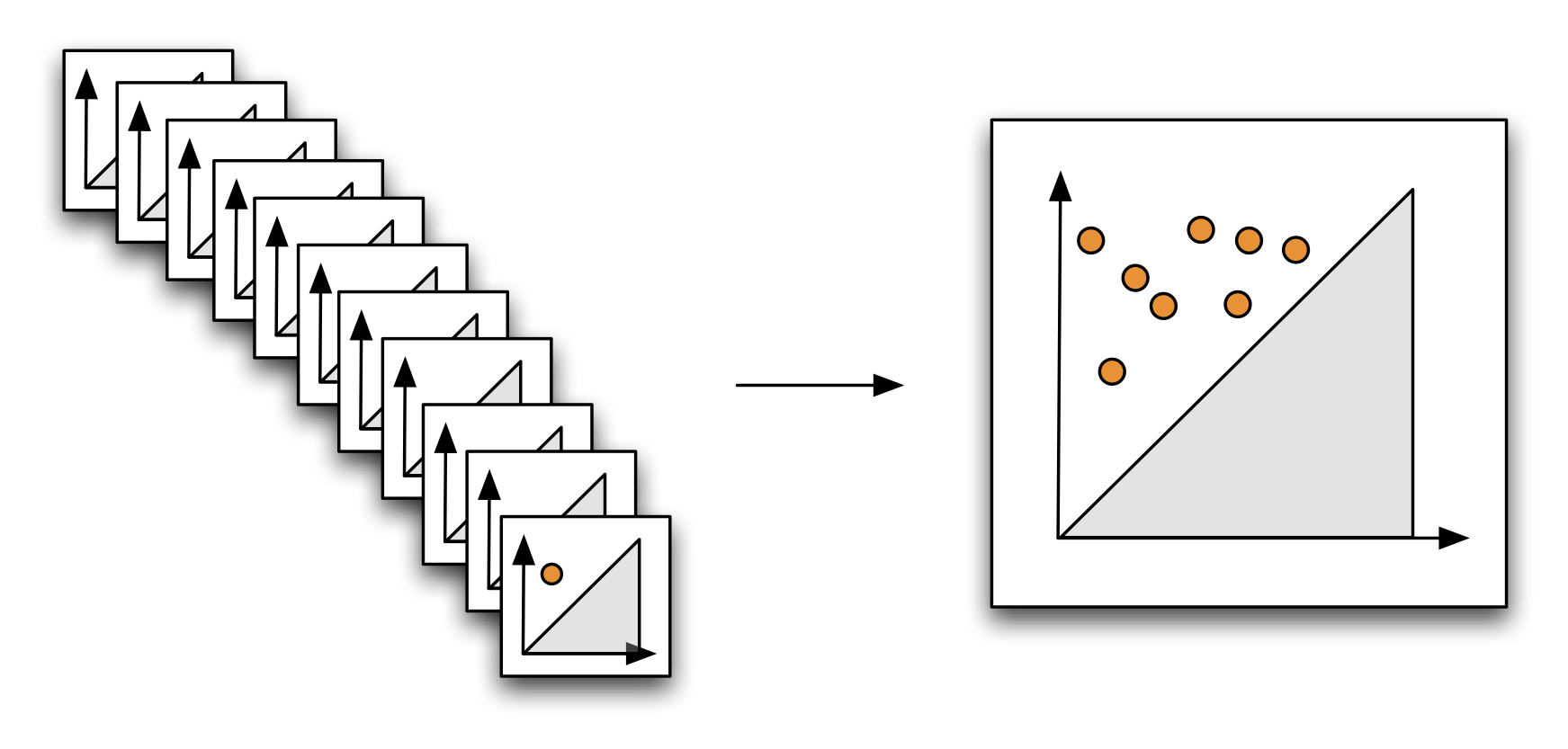
The scripts in the base directory (i.e. Persistence_parallel_dX.m and Persistence_parallel_Ripser.m) compute the principal persistence sets $D_{2k+2,k}^{\mathrm{VR}}(X)$ of a finite metric space $X$. The input is the distance matrix $d_X$ of $X$ stored in a .mat file. The program will load this matrix and sample a large number of $n$-point subsets, where $n=2k+2$.

Example

We have included a file dX_example_circle.mat with 1000 points sampled uniformly at random from the unit circle. As long as you have both Ripser and the Parallel Computing Toolbox installed, both Persistence_parallel_Ripser.m and Persistence_parallel_dX.m should run out of the box. You can further personalize the scripts as described in the Usage section.

Usage

You need to set the following parameters:

1. Store a distance matrix named dX in a .mat file. In order to guarantee meaningful results, the matrix should be square, symmetric, have diagonal 0, and satisfy the triangle inequality.
   • Keep in mind that a reasonable size for dX is at most 5000x5000, depending on your system.
2. Select the script that you want to use (Persistence_parallel_Ripser.m or Persistence_parallel_dX.m). Open the file to set the following book-keeping variables:
   • filename_metric_space: Name (and path) of the .mat file containing the distance matrix.
   • results_file: The name of the file where the results will be stored.
   • save_to_file: Boolean flag to decide if you want to save the output to results_file.mat or if you only want to keep it in Matlab's workspace.
   • temp_file: The ending of the file where the temporary results will be stored. The files are named checkpoints_temp_file_#.mat, where # runs from 1 to the number of cores utilized. This variable is usually not edited, unless you are running several copies of the script at the same time.
   • CoresRequested: The number of cores that you want to use. The maximum is the number of physical cores (not logical cores) available in your system. You can set CoresRequested = 0 to use the default chosen by Matlab.
     • Matlab can only work with physical cores. See https://www.mathworks.com/matlabcentral/answers/80129-definitive-answer-for-hyperthreading-and-the-parallel-computing-toolbox-pct#answer_89845 for a more detailed explanation. In short, logical cores require hyperthreading, but this negatively impacts Matlab's performance more often than not.
3. Set the simulation parameters:
   • dim: The dimension of homology that you want to calculate. The program will automatically set n=2*dim+2 to calculate the principal persistence set.
   • nReps: Number of $n$-point samples to take from $d_X$.
4. Once you've decided on the above parameters, run your selected script from the Matlab command window. This will produce a .mat file containing the results.

Output

The script produces a graph of $D_{n,k}^\mathrm{VR}(X)$, as described in the paper and in the figure above. It also saves the following variables in results_file.mat:

• confs: Matrix of size [n, nReps]. Each column I = confs(:,i) is the set of indices a set of $n$ points sampled from $X$.
• dms: Array of size [n, n, nReps]. Each page dm = dms(:,:,i) is the distance matrix of a sample of $n$ points from $X$. It is obtained from dX and confs by setting I=confs(:,i) and dm=dX(I,I).
• bd_times: An array of size [nReps, 2] with the persistence diagrams of the samples. The first column bd_times(:,1) contains the birth times and the second, bd_times(:,2), the death times. A row bd_times(i,:) will be non-zero if, and only if, the configuration with distance matrix dms(:,:,i) produced persistence homology.

Shape_Analysis

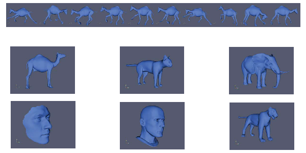
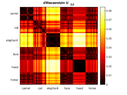
We refer the user to Section 4.3.1 of our paper for the description of the experiment. We used the database from the paper ''Deformation Transfer for Triangle Meshes'' by Robert W. Sumner and Jovan Popović. As of the time of writing, both the database and the paper can be found here: https://people.csail.mit.edu/sumner/research/deftransfer/.

To use this code, download the database from the link above. Place the folders with the meshes in the models directory. To reproduce the experiments in our paper, you should have the following subfolders: camel-poses, cat-poses, elephant-poses, face-poses, head-poses, and horse_poses. Then, run the scripts in the Shape_Analysis folder in order (run S1_Setup, then S2_persistence_Sets.m, and so on). The order is set up so that, if you change parameters in one script, you don't have to re-run every script before it. These parameters are:

• S1_setup.m:
  • nBins0 and nBins1 are the number of points used to approximate $U_{2k+2,k}^\mathrm{VR}(G_i)$ for $k=0$ and $k>0$, respectively. Be aware that the number of points is only guaranteed to be close to nBins0 and nBins1. Choose these numbers so that emd_mex can compute the Wasserstein distance between vectors with that size.
  • NFPS: Number of points in the graphs $G_i$. Choose NFPS so that MATLAB can store a matrix of size [NFPS,NFPS].
• S2_Persistence_Sets.m:
  • Ks: Vector with the dimensions k to compute the persistence sets $D_{2k+2,k}$.
  • nRepsK: Vector of the same size as Ks. The entry nRepsK(idx) is the number of samples to take to compute $D_{2k+2,k}$ for k=Ks(idx). Note: This value is unused when k=0, but nRepsK needs a placeholder value.
• S3_Persistence_Diagrams.m:
  • maxHomDim: We compute the persistence diagrams from dimension 0 up to maxHomDim.
  • nL: We usually can't compute the persistence diagram of the whole set $G_i$. Instead, we operate on a subset of size nL.
  • s_edges: We compute persistence diagrams up to a threshold t chosen so that the 1-skeleton of the Vietoris-Rips complex contains a certain percentage of the total number of edges. That percentage is 0 < s_edges < 1.
• S4_NN_Classification.m:
  • nTests: The number of times that the 1-nearest neighbor experiment will be repeated.
• S5_NN_Classification_dWmax.m:
  • nTests: Same as in S4_NN_Classification.m.
  • Line 88: You can modify the initial guess w0 here.

Other_Examples

We include a folder with further experiments.

Ellipses

The script Persistence_Single_Ellipse.m computes the principal persistence set of an ellipse in $\mathbb{R}^2$ with semiaxes $a$ and $b$. You can modify the variables k, nReps, save_to_file, and results_file as above. This code is not parallelized. Additionally, you can modify the length of the semiaxes a and b. The variable confs now has size [n, 2, nReps], and each page confs(:,:,i) is an $n$-point subset of $\mathbb{R}^2$. Points are stored as row vectors. We include example calculations for some combinations of a and b.  a=1.2, b=1.0.png?raw=true "D41_Ellipse") An image similar to the above can be produced by running Persistence_Single_Ellipse.m with a=1.2, b=1, k=1, and nReps=10^6.

Graphs

These scripts compute principal persistence sets of metric graphs. For the script Persistence_Metric_Graph.m, the input is a weighted adjacency matrix stored in the variable A. We include several examples (commented in the file). Persistence_Metric_Graph_Collection.m can operate several graphs at once. The input is a set of weighted adjacency matrices, each separated by an empty line, stored in a text file in the Other_Examples/Graphs/data/ folder. The folder includes several examples.

Similar to the main script, the variables that can be modified in these scripts are k, nReps, save_to_file, and results_file. If you set save_to_file=true in Persistence_Metric_Graph_Collection.m, the script will save the graphs of the persistence sets to the 'Results/' folder instead of showing them on screen.

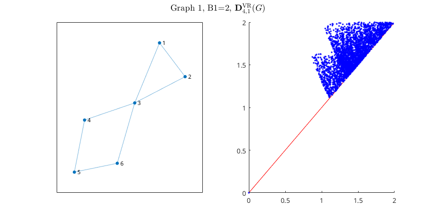The image above was obtained by running Persistence_Metric_Graph.m with k=1 and nReps=10^5. Among the adjacency matrices in the file, we uncommented the one titled "Wedge of two circles of different lengths".

Random_Walk_Sd

We have observed that sampling 6-point configurations from $\mathbb{S}^2$ doesn't yield a good enough sampling of $D_{6,2}(\mathbb{S}^2)$ to determine its boundary. For this reason, we implemented a Markov Chain Monte Carlo random walk biased towards rare configurations. The script Persistence_complete_w_rw.m executes this idea. Choose k and set n=2k+2. To approximate $D_{2k+2,k}^{\mathrm{VR}}(\mathbb{S}^d)$, the script first samples nReps configurations of n points from $\mathbb{S}^d$ and computes the set $D_\text{unif}$ of their persistence diagrams. It then executes a random walk with nSteps steps as follows. It starts with a configuration $X_0$ that has a non-trivial persistence diagram, and defines $D_0 := D_\text{unif}$. At each step $t$, we obtain $X_{t-1}^{\sigma^2}$ by perturbing the previous configuration $X_{t-1}$ with Gaussian noise of variance $\sigma^2$. Let $dgm_{t-1}$ and $dgm_{t-1}^{\sigma^2}$ be the persistence diagrams of $X_{t-1}$ and $X_{t-1}^{\sigma^2}$, respectively. We then compute the cardinalities $N_{\text{pre}} = |B_\epsilon(dgm_{t-1}) \cap D_{t-1}|$ and $N_{\text{post}} = |B_\epsilon(dgm_{t-1}^{\sigma^2}) \cap D_{t-1}|$ (the balls are induced by the bottleneck distance). We accept the new configuration $X_{t-1}^{\sigma^2}$ with probability $\min(1,N_\text{pre}/N_\text{post})$, and set $X_t := X_{t-1}^{\sigma^2}$ and $D_t := D_{t-1} \cup {dgm_{t-1}^{\sigma^2}}$. If $X_{t-1}^{\sigma^2}$ is rejected, we generate a new $X_{t-1}^{\sigma^2}$ by perturbing $X_{t-1}$ until the new configuration is accepted. This causes the random walk to diverge from the diagrams that already are in $D_\text{unif}$ and produces configurations closer to the boundary of $D_{2k+2,k}^\mathrm{VR}(\mathbb{S}^{d})$.

The variables that can be modified in this script are:

• d: The dimension of the sphere $\mathbb{S}^d$.
• sigma: The standard deviation $\sigma$ of the normal perturbation.
• eps: The radius of the balls $B_\epsilon(D_{t-1})$ and $B_\epsilon^{\sigma^2}(D_{t-1})$.
• nReps: Number of $n$-point samples in the initial uniform sampling.
• nSteps: Number of steps that the random walk will take.
• k, CoresRequested, save_to_file, results_file: Same as in the main script.

Output

The scripts produces two sets of variables: confs_0, dms_0, bd_times_0, and confs_n, dms_n, bd_times_n. The the initial uniform sample and the random walk are stored in the variables with subindex 0 and n, respectively. The description of dms_* and bd_times_* is the same as in the main script. The difference is confs_*. In this script, each page confs_*(:,:,i) is an $n$-by-$(d+1)$ matrix representing an $n$-point sample from $\mathbb{S}^d$.

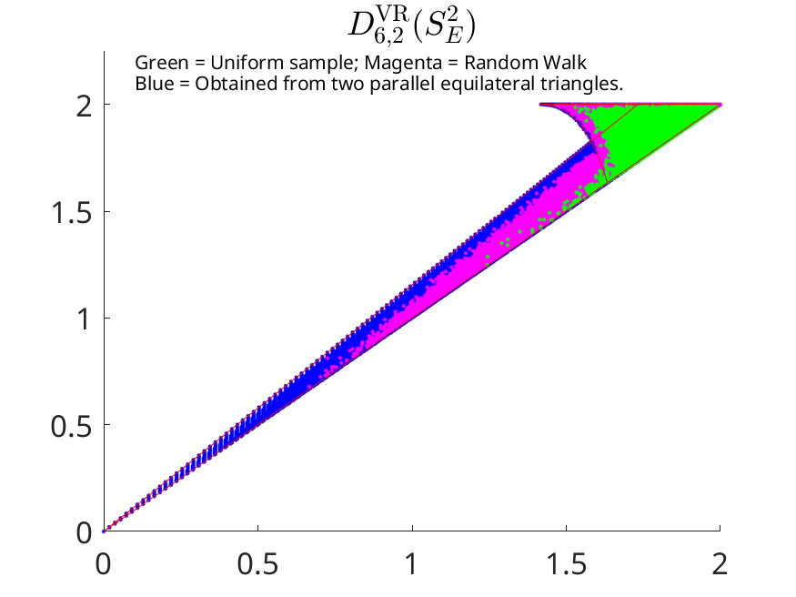An image similar to the above can be produced by running Persistence_complete_w_rw.m and Plot_S2_conjecture.m in succession with the current parameters.

Extra files

The script Persistence_random_walk_plot_progress.m loads a file with a uniform sample of $D_{6,2}^\text{VR}(\mathbb{S}^2)$ and executes the random walk described above. The difference is that it plots $D_{6,2}^\text{VR}(\mathbb{S}^2)$ and highlights the diagrams produced by the random walk as it finds them.

TO DO

• Do we want to save the results to a .mat file directly from Persistence_parallel_*.m, or should we gather the results distributed in the checkpoint_temp_file_*.mat files?
  • For now, we're saving the results directly to a .mat file. The checkpoints are there for redundancy in case the main program crashes.
  • In any case, it would be useful to upload the code that gathers the results from the checkpoints.
• Write a version of Persistence_parallel_Ripser.m that allows for $n > 2k+2$.
• Set a random seed. This is not straightforward with parallel code because each worker has its own random seed.