Construction and analysis of cell-type-specific functional gene network, with SCINET and HumanNetv3
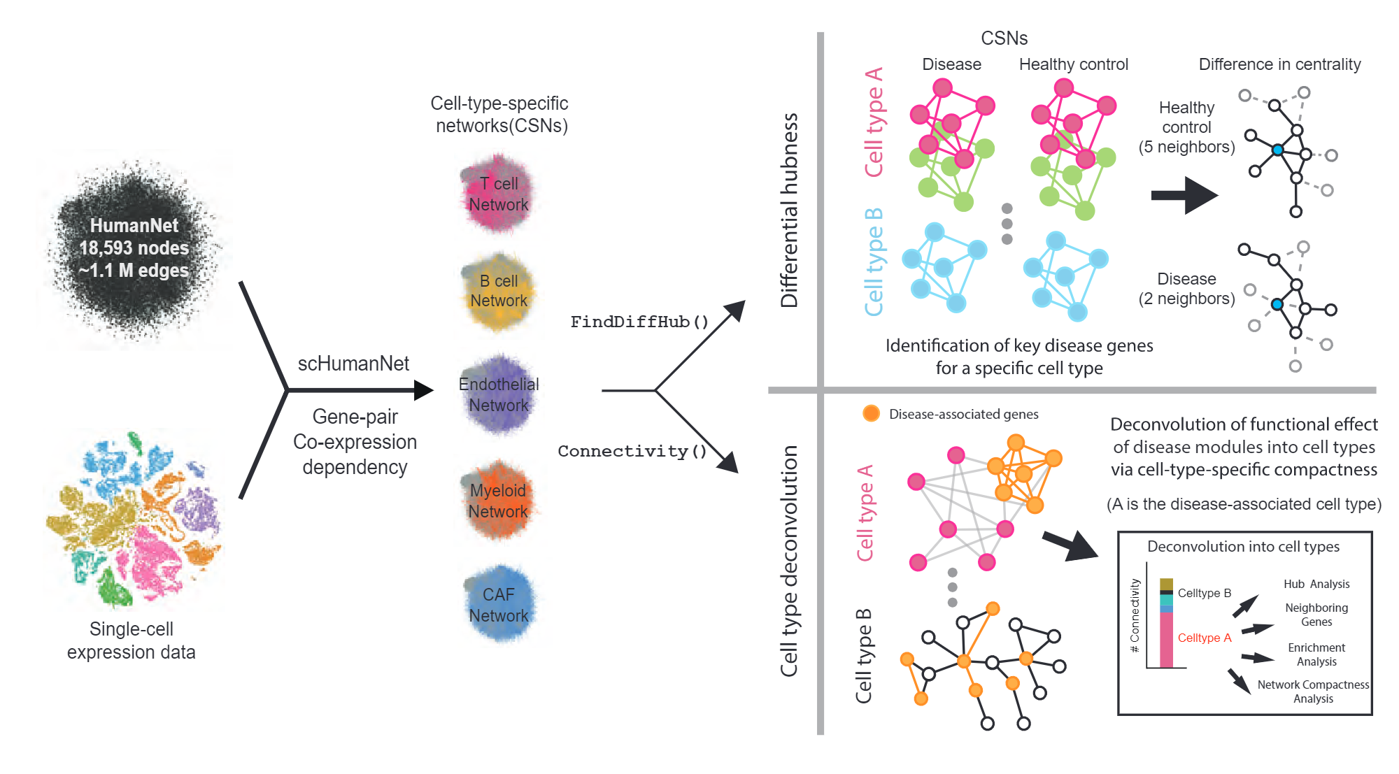
scHumanNet enables cell-type specific networks with scRNA-seq data. The SCINET framework (Mohammade et al. Cell Syst. 2019) takes a single cell gene expression profile and the “reference interactome” HumanNet v3, to construct a list of cell-type specific network. With the modified version of SCINET source code and the detailed tutorial described below, researchers could take any single-cell RNA sequencing (scRNA-seq) data of any biological context (e.g., disease) and construct their own cell-type specific network for downstream analysis.
For a given scRNA-seq data set, the SCINET framework utilize imputation, transformation, and normalization from the ACTIONet package(Mohammadi et al. Nat. Commun. 2018) to robustly capture cell-level gene interactions. HumanNet v3 with 1.1 million weighted edges are used as a scaffold information to infer the likelihood of each gene interactions. A subsampling scheme for each cell-type clusters (cell groups) ensures retaining of accurate gene interaction strength despite the incompleteness of single cell dataset at high resolution. Overall, we show that HumanNet v3 not only allow gene prioritization in broad spectrum of diseases, but through construction of context specific cell-type networks, also allow an in-depth study of disease heterogeneity and its underlying mechanism at a cellular level.
For running scHumanNet, we recommend a conda envrionment to install
packages in the packages folder.
#if this is the first time you are using conda envrionment add following channels for installation of scHumanNet
$ conda config --add channels conda-forge
$ conda config --add channels bioconda
$ git clone https://github.com/netbiolab/scHumanNet.git

$ conda env create -n scHumanNet -f ./scHumanNet/packages/scHumanNet_env.yml
$ conda activate scHumanNet

#check whether appropriate dependencies have been installed
(scHumanNet) $ conda install --file ./scHumanNet/packages/requirements_scHumanNet.txt
Install the modified version of ACTIONet.
(scHumanNet) $ R CMD INSTALL ./scHumanNet/packages/ACTIONet_2.0.18_HNv3Start R and install SCINET and scHumanNet.
devtools::install_github("shmohammadi86/SCINET")
devtools::install_github("netbiolab/scHumanNet")(add Seurat if necessary)
library(scHumanNet)
library(ACTIONet)
library(SCINET)
library(Seurat)
library(igraph)
library(SingleCellExperiment)
library(purrr)
library(dplyr)For the first example case, we showcase the construction of scHumanNet using publically accessible pan-cancer dataset from Qian et al. Cell Research 2020. The 10X count folder and the metadata can be downloaded from http://blueprint.lambrechtslab.org.
counts <- Read10X('/your/path/to/BC_counts/')
meta <- read.table('/your/path/to/BC_metadata.csv', header = T, sep = ',')This tutorial converts count data and metadata to sce obeject from
SingleCellExperiment, to be used as intput for network construction.
data <- SingleCellExperiment(assays = list(logcounts = counts), colData = meta)For seurat objects, manually insert count data and metadata within the
SingleCellExperiment(), or use the as.SingleCellExperiment()
provided in the Seurat package.
data <- SingleCellExperiment(assays = list(logcounts = seurat_object@assays$RNA@counts), colData = seurat_object@meta.data)
data <- Seurat::as.SingleCellExperiment(seurat.object)
Prior to scHumanNet construction, reduce data and use the ace class from
the ACTIONet package. run.ACTIONet() is optional, this wrapper function performs matrix transformation via revese-rank normalization and imputation. For more information, refer to Mohammadi et al. Nat Communication
ace <- reduce.ace(data)
#ace = run.ACTIONet(ace = ace, thread_no = 8)
The column CellType of the metadata here indicates the column where
each barcode is annotated from the user’s preferred choice of methods.
ace[['Labels']] <- meta$CellTypeLoad HumanNetv3 interactome and retrieve cell-type specific interactions. Command data('HNv3_XC_LLS') loads the interactome as an igraph object named graph.hn3.
data('HNv3_XC_LLS')
ace <- compute.cluster.feature.specificity(ace, ace$Labels, "celltype_specificity_scores")
Celltype.specific.networks = run.SCINET.clusters(ace, specificity.slot.name = "celltype_specificity_scores_feature_specificity")
Sort each genepair alphabetically and add LLS weight from HumanNetv3.
Elements of sorted.net.list are stored as edgelist. This is later useful for assessing edge overlap between scHumanNets.
sorted.net.list <- SortAddLLS(Celltype.specific.networks, reference.network = graph.hn3)Check each element of list and save scHumanNets, with both SCINET and LLS weights included in the edgelist for downstream analysis. R code used to analyze pan-cancer scHumanNet is included in the figures folder.
lapply(sorted.net.list, head)
saveRDS(sorted.net.list, './sorted_el_list.rds')
scHumanNet package provides a statistical framework to threshold functional hub genes from each cell-type specific networks via FindAllHub(). Briefly, it creates a null model of random networks by swapping edges with equal probability, thus creating a distribution of centrality values. Each hub's centrality is measured against this null distribution and a p-value is calculated. Default correction method is Benjamini-Hochberg method and the default threshold cut value is FDR < 0.05. To filter for genes, use the gene column and not the rownames.
sig.hub.df <- FindAllHub(sorted.net.list, centrality="degree")
sig.hub.df| Centrality | gene | pvalue | qvalue | celltype |
|---|---|---|---|---|
| 1 | CD19 | 0.0000891981090000892 | 0.00428745577260429 | B_cell |
| 0.9995374 | CD40 | 0.0000891981090000892 | 0.00428745577260429 | B_cell |
| … | … | … | ... | ... |
| 0.9635941 | TRAF3 | 0.00172331258975586 | 0.0463678793681187 | T_cell |
| 0.963206816421379 | LAT | 0.00172331258975586 | 0.0463678793681187 | T_cell |
With scHumanNet we also provide a computaitonal framework to statistically asssess the connectivty of a given geneset at the cellular level of scHumanNets. In this example we use the Immune Checkpoint molecules(ICMs) as a geneset to assess in what celltypes these genesets have strong co-functional characteristic. In common cases user may use a DEG derived genesets or bulk sample derived signatures genes to find whether the genesets' cofunctionality is supported constructed scHumanNet models.
The output of Connectivity() is a list with three elements: 1. the null distribution vector of selected random gene's connectivity. 2. non-parametric pvalue of the user-input geneset. 3. geneset vector that was detected in the input scHumanNet.
data("ICMs_auslander")
icm.connectivity <- DeconvoluteNet(network = sorted.net.list, geneset = icm.genes)
icm.connectivity.tcell <- Connectivity(network = sorted.net.list[["T_cell"]], geneset = icm.genes, simulate.num = 10000)

#we can also perform a conncectivity test for all scHumanNets. this will take some time...
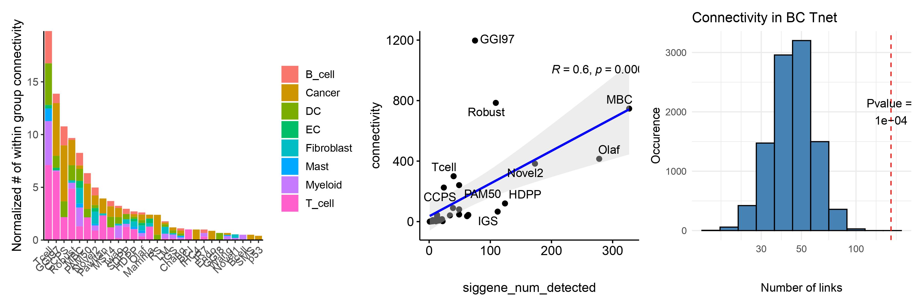
icm.connectivity.nulltest.list <- lapply(sorted.net.list, function(net){Connectivity(network = net, geneset = icm.genes, simulate.num=10000)})Of note, we can also compare the functional connectivity of multiple genesets. In this case, the geneset is provided as a named list for parameter geneset of DeconvoluteNet(). In this case the output dataframe contains column Connectivity number normlalized for the length of detected signatures. It is often informative to find which geneset have the most co-functional properties by utilizing scatter plots. Here we show that in the breast cancer signature genesets, signature GGI97, Robust, Tcell have most connectivity. In practice, this function can be potentially used to deconvolute previously identified genesets and analyze the cellular context of co-functionality of user's scRNA seq dataset.
It is often times useful to see which geneset has most co-functionality. We show in the example here that geneset GGI97, Robust, Tcell is the most cofunctional geneset when assessed for their connectivty in the entire HumanNetv3 interactiome compared to the numeber of geneset. For detailed use of the reference interactome, please refer to the HumanNetv3 Web Server.
library(ggpubr)
library(ggplot2)
library(ggrepel)
library(patchwork)

data("BC_signatures")
bcsig.connectivity <- DeconvoluteNet(network = sorted.net.list, geneset = bc.sig.list)


#get sum of connectivity for each signature
connectivity.sum <- with(bcsig.connectivity,tapply(connectivity.normalized,signature_name,FUN=sum))
mylevels <- names(connectivity.sum[order(connectivity.sum, decreasing = T)])

bcsig.connectivity$signature_name <- factor(bcsig.connectivity$signature_name, levels = mylevels)

p1 <- ggplot(bcsig.connectivity, aes(x=signature_name, y=connectivity.normalized, fill=scHumanNet))+
  geom_bar(position = 'stack', stat = 'identity') +
  theme_classic()+
  theme(
    panel.grid=element_blank(),
    legend.text=element_text(size=10),
    text = element_text(size=12),
    legend.title = element_blank(),
    axis.title.x = element_blank()
  )+
  ylab("Normalized # of within group connectivity")+
  xlab("Breast Cancer prognostic signatures") +
  rotate_x_text(45) +
  scale_y_continuous(expand = c(0, 0))


hnv3.connectivity.sig <- GenesetHnv3(geneset = bc.sig.list)

p2 <- ggscatter(hnv3.connectivity.sig, x = "siggene_num_detected", y = "connectivity",
                label = "name", repel = TRUE,
                add = 'reg.line', conf.int = T,
                add.params = list(color='blue', fill = 'lightgray')) +
  stat_cor(method = "pearson", label.x = 200, label.y = 1000)
Finally with the Connectivity() user can assess whether their geneset's connectivity is statistically enriched compared to a random model. the random model is contructed via rejecion sampling where topological similar set of random nodes are slected and assessed for their connectivity. Here, we test the connectivity of geneset GGI97 in Breast Cancer Tcell, and show that it is statiscally significant.
ggi.genes <- bc.sig.list[["GGI97"]]
tnet.ggi <- Connectivity(network = sorted.net.list[["T_cell"]], geneset = ggi.genes, simulate.num = 10000)
tnet.ggi[["p.value"]]

p3 <- ggplot() + aes(tnet.ggi[["null.distribution"]])  +
  geom_histogram(binwidth=0.1, colour="black", fill="steelblue") +
  scale_x_continuous(trans='log10') +
  theme_minimal() +
  ggtitle('GGI Connectivity in BC Tnet') +
  ylab('Occurence') + xlab('Number of links') +
  geom_vline(aes(xintercept=tnet.ggi[["observed"]]), colour="red", linetype="dashed") +
  geom_text(aes(tnet.ggi[["observed"]], 2000, label = paste0("Pvalue = \n",tnet.ggi[["p.value"]])))


p1+p2+p3
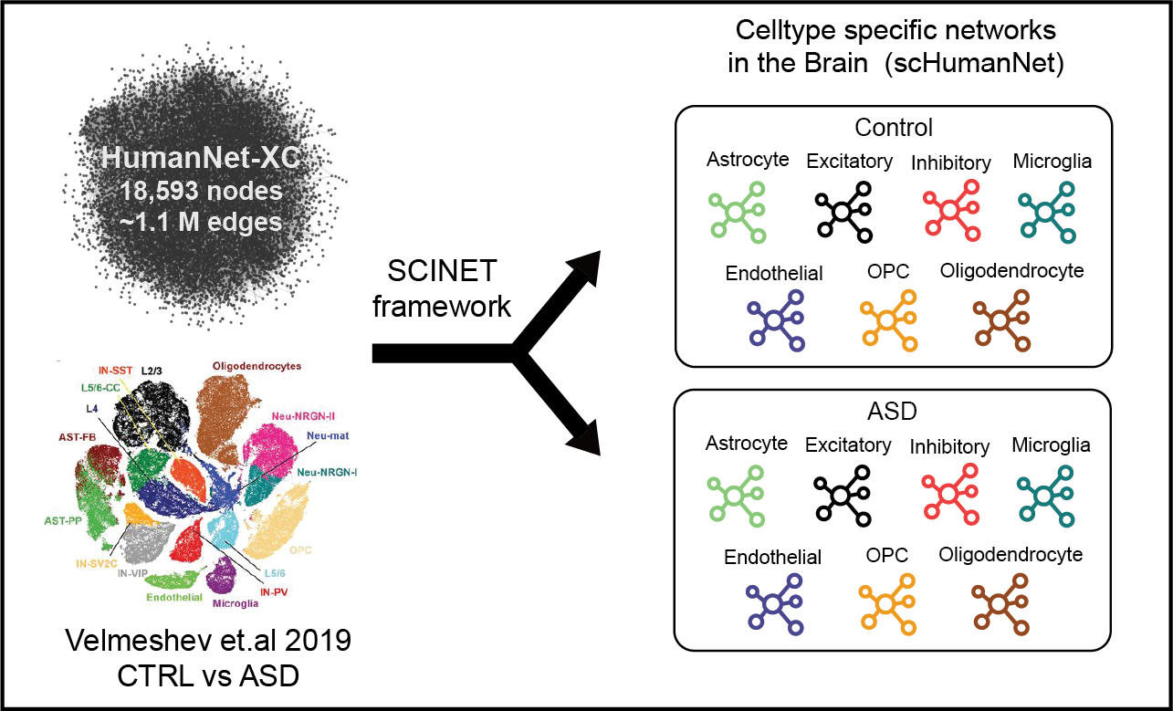
In this example we provide a framework for a common downstream network analysis, identification of differential hub in a control vs disease scRNA-seq study. Here we present an example cell-type-specific gene prioritization associated with ASD. Differential hub gene is identified that significantly differs in centrality for each neuronal celltypes of healthy vs ASD scHumanNet(data derived from Velmeshev et al. Science 2019).
Download the publically accessible data meta.txt and 10X folder from
https://autism.cells.ucsc.edu.
counts <- Seurat::Read10X('/your/path/to/10X_out/')
meta <- read.table('/your/path/to/meta.txt', header = T, sep = '\t')

#check if barcodes match
rownames(meta) <- meta$cell
meta$cell <- NULL
identical(colnames(counts), rownames(meta))

#merge annotated celltypes to larger granularity
#neu_mat, NRGN neurons are seperated and will be excluded because it is either similar to Excitatory neurons based on UMAP analysis and is thus considered ambiguous
meta$celltypes_merged <- ifelse(meta$cluster %in% c('AST-FB','AST-PP'), 'Astrocyte',
                                ifelse(meta$cluster %in% c('IN-PV', 'IN-SST','IN-SV2C', 'IN-VIP'), 'Inhibitory',
                                       ifelse(meta$cluster %in% c('L2/3', 'L4', 'L5/6','L5/6-CC'), 'Excitatory',
                                              ifelse(meta$cluster %in% c('Neu-mat','Neu-NRGN-I', 'Neu-NRGN-II'), 'Others',
                                                     as.character(meta$cluster)))))
To make a control vs disease network for each celltype we make a new
column that combines celltype and disease annotation For the Velmeshev
2019 data, column name diagnosis and celltypes_merged includes
disease and celltype annotation respectively.
meta$celltype_condition <- paste(meta$diagnosis, meta$celltypes_merged, sep = '_')Construct celltype specific networks for control and disease similarly as above.
data <- SingleCellExperiment(assays = list(logcounts = counts), colData = meta)
ace = reduce.ace(data)
ace[['Labels']] <- meta$celltype_condition
ace = compute.cluster.feature.specificity(ace, ace$Labels, "celltype_specificity_scores")
Celltype.specific.networks = run.SCINET.clusters(ace, specificity.slot.name = "celltype_specificity_scores_feature_specificity")
Add LLS weight from HumanNetv3 for downstream analysis.
data('HNv3_XC_LLS')
sorted.net.list <- SortAddLLS(Celltype.specific.networks, reference.network = graph.hn3)
In this tutorial we will select degree, sum of all weights connecting
the node, as a centrality measure to prioritize genes. The function
GetCentrality also supports betweenness, closeness, and eigenvector
centrality as well.
strength.list <- GetCentrality(method='degree', net.list = sorted.net.list)Percentile rank is used to account for netork size differences. For every gene in the reference interactome, if a node is not existent in the scHumanNet, 0 value is assigned.
rank.df.final <- CombinePercRank(strength.list)Get top 50 central genes for each celltype
top.df <- TopHub(rank.df.final, top.n = 50)
head(top.df)| ASD_Astrocyte | ASD_Endothelial | … | Control_Others |
|---|---|---|---|
| ALDH1L1 | CD4 | … | COX4I1 |
| SLC27A1 | STAT1 | … | UQCRC1 |
| … | … | … | … |
| PAX6 | CD14 | … | COX6B1 |
Get the differential percentile rank value for each genes with function
DiffPR(), where the output is a dataframe with genes and the
corresponding diffPR value for each scHumanNets. The input of DiffPR
includes the output of CombinePercRank(), metadata, column name of the
annotated celltypes and condition(disease & control), and of the two
annotation which will be used as a control. This example dataset
diagnosis contains Control and ASD, and the column
celltypes_merged stores the annotated celltypes.
diffPR.df <- DiffPR(rank.df.final, celltypes = 'celltypes_merged', condition = 'diagnosis', control = 'Control', meta = meta)
head(diffPR.df)| Astrocyte | Astrocyte_ASD-Control | … | Others | Others_ASD-Control |
|---|---|---|---|---|
| AR | -1.0000000 | … | UQCRC2 | -0.9993515 |
| FASN | -0.9996066 | … | TFAM | -0.9990272 |
| … | … | … | … | … |
| ACAA1 | 0.9967962 | … | BCS1L | -0.9951362 |
Finally, we provide two methods to prioritize genes. The first is the nonparametric, statistical method to filter differential hubs
with the function FindDiffHub(). Input requires the output of DiffPR,
and the user-defined pvalue threshold. The output consists of a gene
column, diffPR value sorted from negative to positive value, pvalue, and
the celltype. To extract genes, use the gene column instead of
rownames().
diffPR.df.sig <- FindDiffHub(rank.df.final = rank.df.final, celltypes = 'celltypes_merged', condition = 'diagnosis', control = 'Control', meta = meta, net.list=sorted.net.list, q.method='BH', centrality="degree")
diffPR.df.sig| Control_scHumanNet | Disease_scHumanNet | gene | diffPR | pvalue | qvalue | celltype | |
|---|---|---|---|---|---|---|---|
| ALDH1L1 | 0.9992135 | 1.0000000 | ALDH1L1 | 0.0007864727 | 9.982880e-01 | 0.999598937 | Astrocyte |
| SLC27A1 | 0.9980338 | 0.9995997 | SLC27A1 | 0.0015658614 | 9.971936e-01 | 0.999598937 | Astrocyte |
| … | … | … | … | … | … | … | … |
| C12orf71 | 0.0012836970 | 0 | C12orf71 | -0.0012836970 | 0.9972975 | 0.9996602 | Others |
| ZNF222 | 0.0009627728 | 0 | ZNF222 | -0.0009627728 | 0.9981590 | 0.9996602 | Others |
The second, is to extract top n percent of diffPR genes with the function TopDiffHub(). Input requires the output of DiffPR(),
and the user-defined top_percentage threshold (default 0.05). The output consists of a gene
column, diffPR value sorted by absolute value, the top percengate value, and
the celltype. To extract genes, use the gene column instead of
rownames().
diffPR.df.top <- TopDiffHub(diffPR.df, top.percent = 0.05)
diffPR.df.top| gene | diffPR | top_percentage | celltype | |
|---|---|---|---|---|
| TRIM21 | TRIM21 | -0.8537161 | 0.04973245 | Astrocyte |
| FOXH1 | FOXH1 | -0.8568620 | 0.04910293 | Astrocyte |
| … | … | … | … | … |
| COX16.1 | COX16 | 0.9793814 | 0.007617547 | Others |
| MAP2K1.1 | MAP2K1 | 0.9888977 | 0.003414762 | Others |


