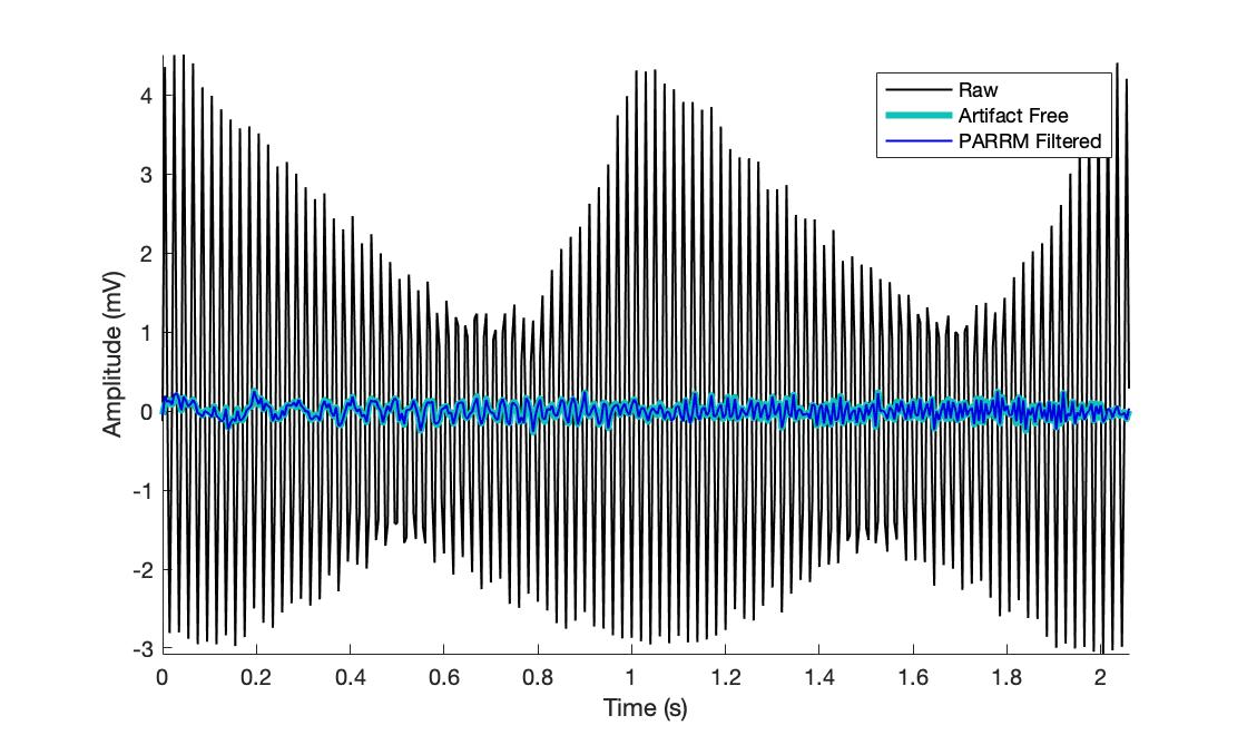
This method operates on the assumption that the artifact is semi-regular, periodic, and linearly combined with the signal of interest.
- The first step is finding the period of the artifact in the raw signal. This is done using a grid search centered about the quotient of the sampling rate and stimulation frequency.
- In order to evaluate each period, samples are translated onto the timescale of the period by finding the modulo of each sample number with the current period of interest.
- Then, using linear regression, the best fitting sum of sinusoidal harmonics of the period is found and the mean squared error of the fit with the raw data is computed.
- The period which minimizes this mean squared error is then chosen.
- This period is used to produce a linear filter that takes four parameters in addition to the period itself: the window size, the skip size, the period distance, and the window direction. Only samples within the window size are used to filter the data at each sample. Samples within the skip size are not used for filtering. Only samples within the period distance on the timescale of the period are averaged together. The window direction is used to specify whether the window only takes past, future, or both into account.
- The linear filter is then applied to the data in order to remove the artifact.
Window size should be chosen based on an estimate of the timescale on which the artifact shape varies. If this is unknown, a power spectral density can be computed and this parameter can be tuned until desirable attenuation of artifactual peaks is achieved.
Skip size is present to account for possible overfitting. If there is a known neural signal on a specified timescale, skip size should be used to ignore samples which may occur within that range of time.
Period distance should be based on the timescale of changes in the artifact waveform. One method to do this is to plot the data on the timescale of the period (found using FindPeriodLFP.m) and determine a timescale over which features are relatively constant. This plot can be produced using the following line of code:
plot(mod(1:length(data)-1,Period),diff(data),'o')
Additionally, there is a script provided in ParamSelection.m that displays a GUI for exploring the effects of PARRM parameters to help with selection. The left subpanel of the figure shows all samples in the data on the timescale of the period, while the right subpanel shows the original and PARRM filtered timeseries. Window size can be adjusted using the slider in the bottom left and PeriodWith corresponds to half the width of the x-axis (zooming in or out will alter the period width). The selected window in the left plot will provide an idea of the variability of the samples used to make a prediction of the artifact as well as how many samples will be used for the prediction. The right panel will provide an indication for how the artifact is being removed from the data.
An example of how to use PARRM for a simulated LFP file is included in demo.m and will produce the following figures:

