This is a Julia implementation of the Fast Parzen Window Density Estimator described in
X. Wang, P. Tino, M. A. Fardal, S. Raychaudhury and A. Babul, "Fast parzen window density estimator," 2009 International Joint Conference on Neural Networks, 2009, pp. 3267-3274.
This is a technique for estimating a probability density from an observed set of data points. The data space is partitioned in hyper-discs of fixed radii r and each partition is modelled with a Gaussian density. The final model is a mixture of Gaussians with each Gaussian fitted locally to a partition.
The algorithm presented in the paper has two versions called 'hard' and 'soft'. This repository provides an implementation of the 'soft' version.
Apart from cloning, an easy way of using the package is to switch into "package mode" with ] in the Julia REPL and use add FastParzenWindows.
There are two functions of interest: fpw and cvfpw.
fpwtakes two arguments, a N×D data matrixXand a scalarrwhich expresses the radius of the hyper-discs in which the data space is partitioned. The output is an object of the typeDistributions.MixtureModel.cvfpwtakes two arguments, a N×D data matrixXand a range of candidate radii of the hyper-discs. It performs cross-validation for each candidaterand returns a matrix of out-of-sample log-likelihoods of dimensions (number ofrcandidates)×(number of folds).
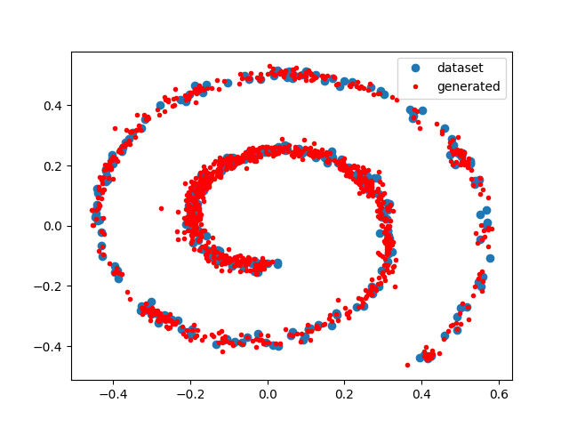
We use a dataset taken from the paper. We generate 300 data points using:
using FastParzenWindows
using PyPlot # must be independently installed, needed only for plotting present example
using Statistics

X = spiraldata(300)

plot(X[:,1], X[:,2], "bo", label="dataset")
We want to find out which r works well for this dataset:
# define range of 100 candidate radii
r_range = LinRange(0.01, 2.0, 100)

# perform cross-validation
cvresults = cvfpw(X, r_range)

# which is the best r?
r_perf = mean(cvresults, dims=2)
best_index = argmax(r_perf)

r_best = r_range[best_index]
Estimate final model:
mix = fpw(X, r_best)

# generate observations and plot them
x = rand(mix, 1000)'
plot(x[:,1], x[:,2], "r.", label="generated")
legend()

