This repository contains C++ classes with the examples in order to solve different numerical problems, related both to physics and math.
ROOT Cern installation is required to run the code.
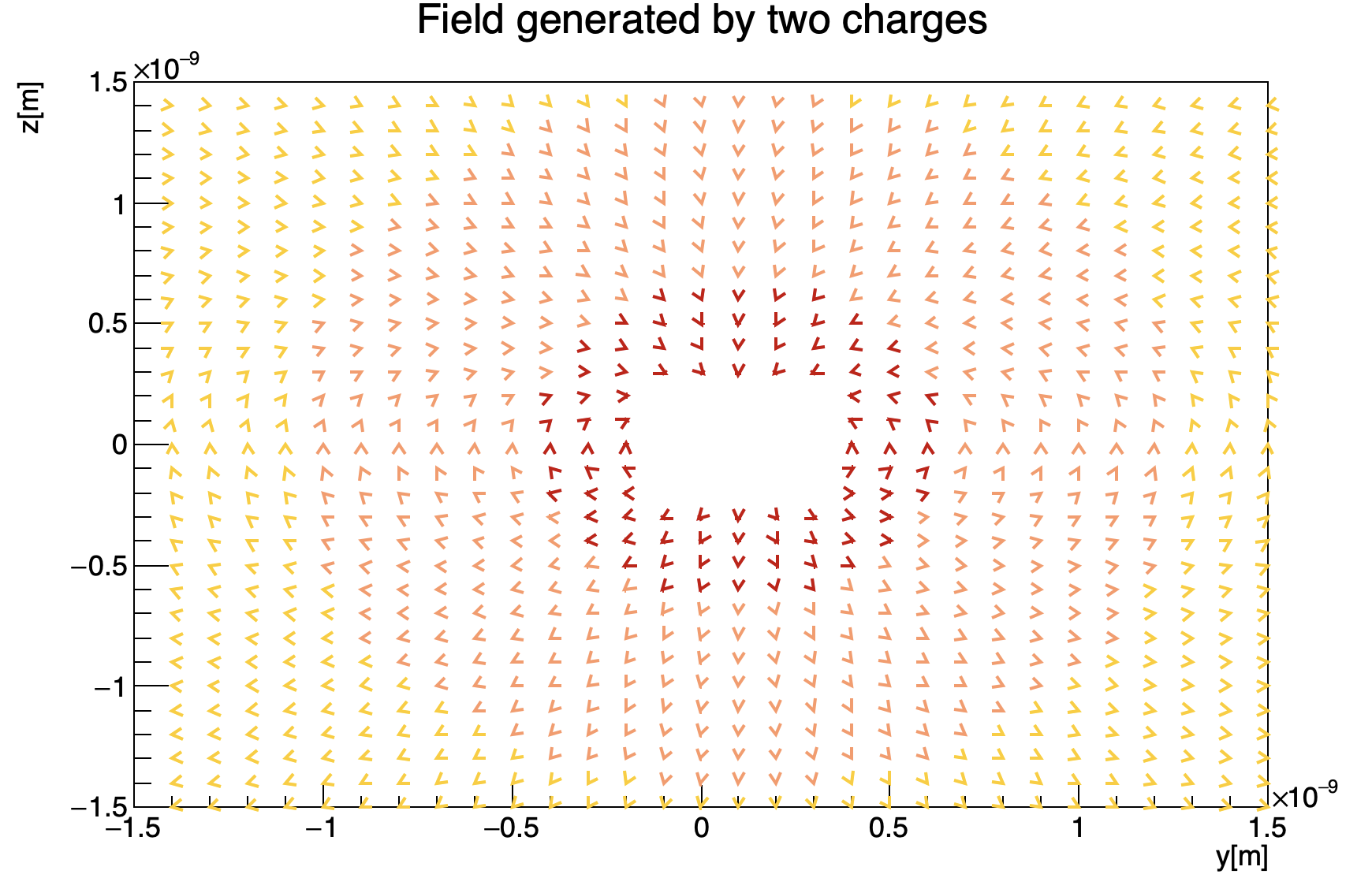
In dipole_electric_field we generate an electric dipole made up by a proton and an electron separated by a distance of an amstrong. Given the position of the dipole, the code computes the trend of the electric field generated as a function of the distance from the dipole. Moreover, we provide the plot of the corresponding field as in figure below:
The folder root_finding provides a class solver and the corresponding method bisection to compute the root of a given function. In particular, functions can be implemented by inheriting from the abstract class funcbase and implementing the specific method eval.
The provided example in main finds the roots of the function f(x) = 3x2+5x-2. To do so, it receives from command line the extremes of the interval and the desired precision.
The folder integrals provides a class integral and the corresponding methods to compute the integral of a given function, functions should be implemented as classes inheriting from funcbase. We implemented the following methods: mid-point, Simpson, trapezoid, each of which is available both with fixed precision and with fixed number of iterations.
The example in main computes the integral of the function sin(x) in [0,π].
The folder diff_equations provides three examples of usage of Euler and Runge-Kutta methods in physical problems. In particular, we provide a graphical solution to the simple armonic oscillator problem, and to the oscillator in presence of an external force.
An example of solution to the harmonic oscillator with an external force is shown in figure below:
While the comparison between the two methods on the simple oscillator is shown in figure below:
The folder montecarlo_integrals provides examples of how it is possible to compute pseudo-random numbers and how random number generation can be used to compute the integral of a function.
In particular, we provide different examples:
- random_numbers: code that implements generators for uniform, gaussian (Box-Muller and accept-reject) and exponential distributions;
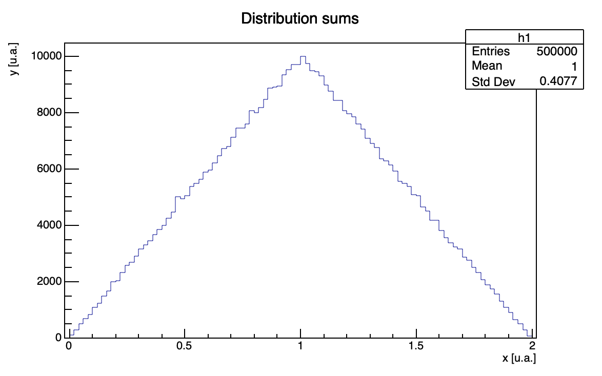
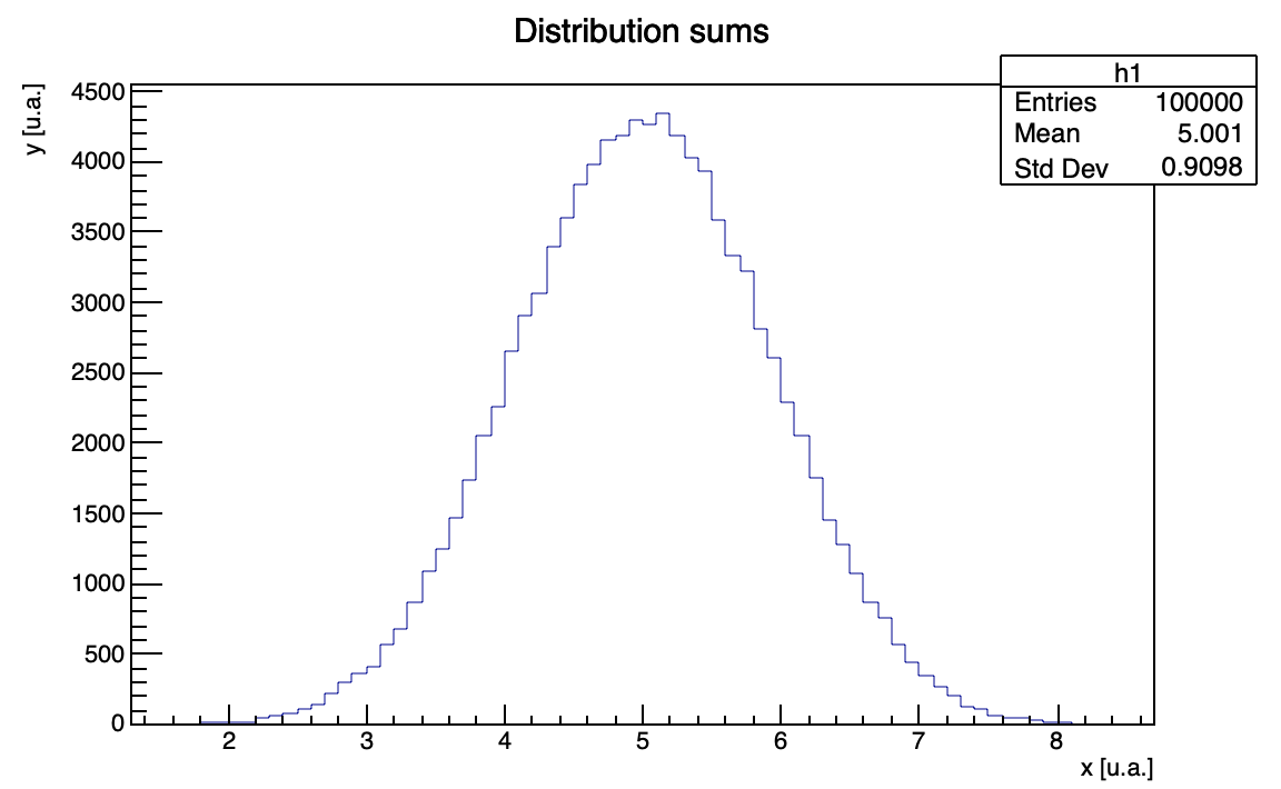
- central_limit_theorem: code that generates a series of random numbers uniformly distributed in [0,1] and computes the sum over a fixed number of elements, in order to directly verify the central limit theorem;
- integrals: class to solve the integral of a function using Monte Carlo methods: mean and hit-or-miss.
- multi_dim_example: example of usage of the Monte Carlo method of the mean in a multi-dimensional problem.
Central limit theorem verification is shown in figures below. Summing 2 variables we obtain the following distributions:
Summing 10 variables we obtain the following distributions:
The folder simulation provides an example of usage of the Monte Carlo method to simulate the results of a specific experiment, by using the same structure of the code, the same approach can be generalized to other experiments.
The refractive index is given by Cauchy relation: n(lambda) = (A + B*lambda^2)^0.5 The real experiment is based on measuring the refractive index of a prism for different wavelengths, in order to provide an estimation of the parameters A and B.
Our simulation is based on the following steps:
- method execute: we generate random values for the measurable quantities given a mean and an error (standard deviation);
- method analyze: we compute all the quantities that should be computed from the measured quantities, exactly as we would do in the real experiment.
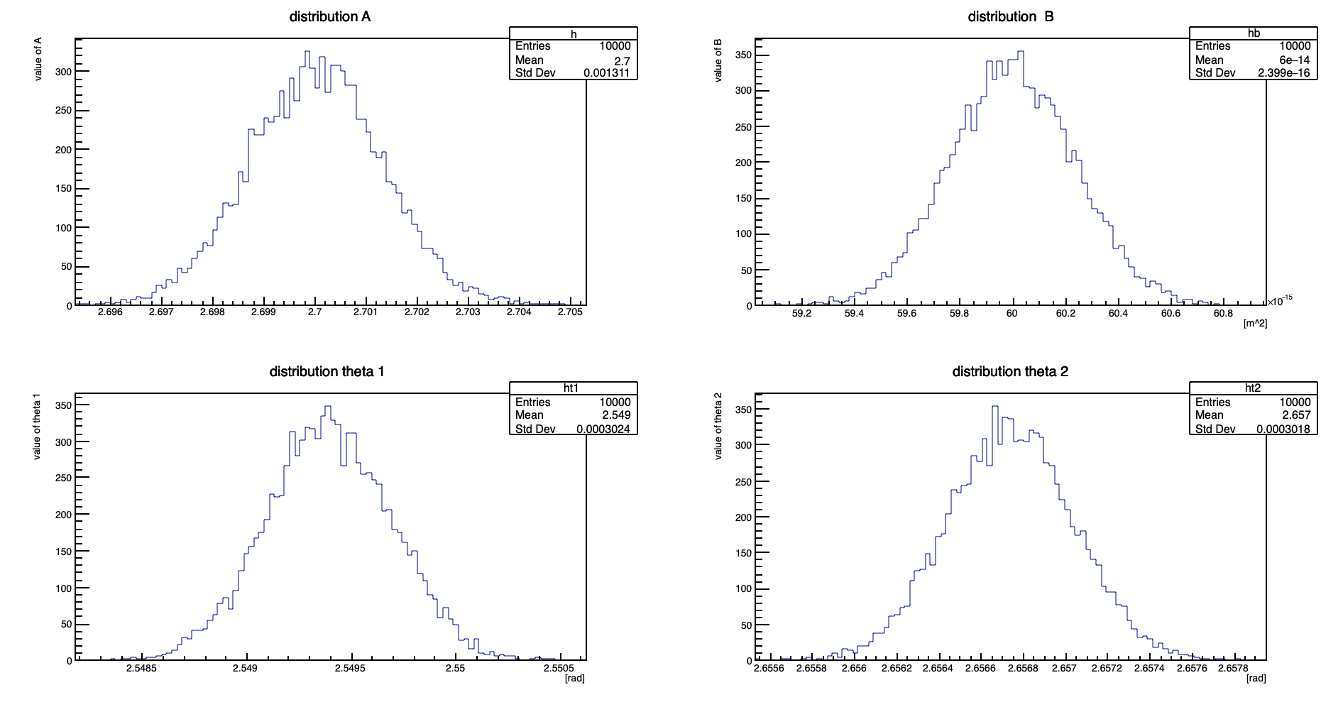
We also study the correlation between the measured quantities and the computed quantities and the error of the computed quantities. Examples of possible plots are shown in figures below. Correlations between residues for different quantities:
Distribution of computed quantities:
Distribution of the error of the computed quantities:
For further reading, see (in italian): TNDS lab


