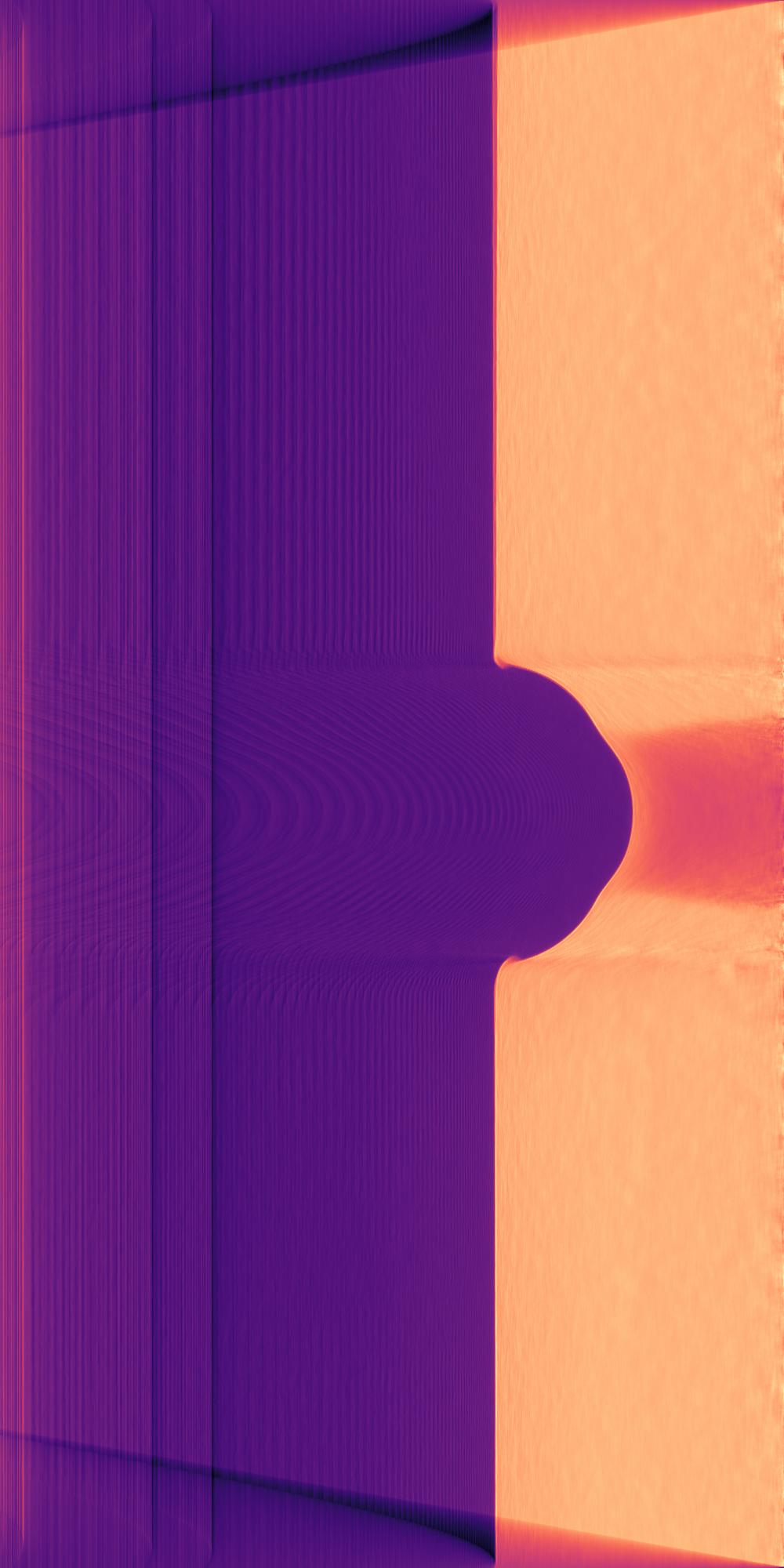
Tomographic reconstruction of axisymmetric fields acquired by a cone beam
Explore the docs »
This python package provides tools for axis-symmetric cone-beam computed tomography. A Feldkamp David Kress algorithm performs the reconstruction which have been adapted such that is exploits the axis-symmetric nature of the tomogram.
This toolkit has a highly specialised usage, and there are plenty of more general and excellent frameworks for tomographic reconstruction, such as:
- TomoPy (General computed tomography, cone and parallel beam geometry)
- PyAbel (Computed tomography based on the inverse Abel transform, parallel beam geometry)
This project aims at providing a simple, accessible toolkit for forward-projection and reconstruction of axis-symmetric tomograms based on a conical beam geometry.
This project is heavily based on the following packages:
To get a local copy up and running follow these steps.
The toolkit is available via PIP, and the instructions below shows how a virtual environment can be created and the toolkit installed.
Prerequisites:
This toolkit is tested on Python 3.6
We recommend the use of virtualenv
Installing:
$ virtualenv -p python3.6 env
$ source ./env/bin/activate #On Linux and Mac OS
$ env\Scripts\activate.bat #On Windows
$ pip install axitom
Now the toolkit is installed and ready for use.
Run the tests:
$ nosetests axitom
If you want to check out the examples, then download the files in the examples folder and run the examples.
These instructions will get you a copy of the project up and running on your local machine for development and testing purposes.
Prerequisites:
This toolkit is tested on Python 3.6
We recommend the use of virtualenv
Clone this repo to your preferred location
$ git init
$ git clone https://github.com/PolymerGuy/axitom.git
We recommend that you always use virtual environments, either by virtualenv or by Conda env
$ virtualenv -p python3.6 env
$ source ./env/bin/activate #On Linux and Mac OS
$ env\Scripts\activate.bat #On Windows
$ pip install -r requirements.txt
You can now run an example::
$ python <path_to_axitom>/examples/comparison_to_Nikon.py
The tests should always be launched to check your installation. These tests are integration and unit tests.
If you cloned the repo, you have to call pytest from within the folder
$ pytest
Let us now go through the necessary steps for doing a reconstruction of a tomogram based on a single image. First, we need to import the tools
import axitom as tom
from scipy.ndimage.filters import median_filter
Assuming that the example data from the repo is located in the example_data folder, we can make a config object from the .xtekct file
config = tom.config_from_xtekct("./example_data/R02_01.xtekct")
We now import the radiogram
radiogram = tom.read_image(r"./example_data/R02_01.tif", flat_corrected=True)
and we remove the top and bottom of the image. This is necessary in this example, as the fixtures will interfere with the algorithm used to find the centre of rotation
 radiogram[:250, :] = 0.95
 radiogram[1800:, :] = 0.95
As we will use a single radiogram only in this reconstruction, we will reduce the noise content of the radiogram by employing a median filter. Using such a filter works fine since the density gradients within the specimen are relatively small. You may here choose any filter of your liking.
radiogram = median_filter(radiogram, size=20)
Now, the axis of rotation has to be determined. The axis of rotation is found by first binarizing of the image into object and background, and subsequently determining the centre of gravity of the object
_, center_offset = tom.object_center_of_rotation(radiogram, config, background_internsity=0.9)
The config object has to be updated with the correct values
 config.center_of_rot_y = center_offset
 config.update()
We are now ready to initiate the reconstruction
tomo = tom.fdk(radiogram, config)
The results can then be visualized
import matplotlib.pyplot as plt
plt.title("Radial slice")
plt.imshow(tomo.transpose(), cmap=plt.cm.magma)
Contributions are what makes the open-source community such a fantastic place to learn, inspire, and create. Any contributions you make are greatly appreciated.
- Fork the Project
- Create your Feature Branch (
git checkout -b feature/AmazingFeature) - Commit your Changes (
git commit -m 'Add some AmazingFeature) - Push to the Branch (
git push origin feature/AmazingFeature) - Open a Pull Request
Distributed under the MIT License. See LICENSE for more information.
Sindre Nordmark Olufsen (PolymerGuy) - sindre.n.olufsen@ntnu.no
We are in great debt to the open-source community and all the contributors the projects on which this toolkit is based.


