nimarb/random-nas-combined

Using Random NAS to Evaluate Disortion Robustness of CNN Architecture Types

This code was used to explore the fundamental differences between the DNN architecture types VGG, ResNet, and DenseNet.

Random NAS is used to create random structures of the three DNN types and then test them for their performance. Specifically, we look at the performance when trained on small training datasets and the networks robustness against distortions.

Running the Code

To be able to run the code using the two methods stated below, you have to create the folders log and save_dir in the current directory.

Locally

The experiment's main function is contained in exp_main.py. However, we suggest to run the code through the yagi_rnd_nas_cli.py file if your machine has multiple GPUs to take advantage of them. For example, to run a DenseNet experiment on multiple GPUs, you can use:

python3 yagi_rnd_nas_cli.py --run_type local --num_train 50000 --archs_per_task 38 --arch_type densenet --num_min_depth 2 --num_max_depth 7

That would start the experiment with the DenseNet architecture on your local computer. It would use all available GPUs and try 38 different architectures per GPU. All architectures would have between 2 and 7 layers (inclusive) and are trained on 50k training images of CIFAR10.

On a Server (qsub)

python3 yagi_rnd_nas_cli.py --run_type qsub --num_train 25000 --archs_per_task 20 --arch_type resnet --server_names yagi11 yagi12 yagi13 --file_to_run yagi_rnd_nas_resnet_archs.sh

Basically almost identical to the local command. When selecting --run_type qsub, training will be started on all machines provided in the --server_names list. Important: for this to work the provided server names must be in your host file and you must have a valid SSH key without password promt for the servers (either unencrypted or provided via ssh_agent etc). In this case, the script checks for the number of available GPUs on each server and then executes --archs_per_task number of trail runs on each available GPU.

Interpreting Results

The log files are stored in ./log/* but don't contain any information used for evaluation, rather they are just for debugging/verification/process monitoring.

The results are stored in ./save_dir/*, with one folder for each process, i.e. each GPU. accuracies.json contains all recorded accuracies for all runs per process. config.json contains the configuration used for that run. log-active.txt contains the layer structure used and the number of total layers per layer structure. The number of layers is incorrect in config.json.

Consolidating Results

To consolidate the results of one type of run when wanting to plot a graph for all ResNet runs for example, there is a script in create_consolidated_results_json.py. To get a consolidated results file for all ResNet runs for example, run:

$ python3 create_consolidated_results_json.py --arch_type resnet
Saved the consolidated results json to vgg.json

Plotting Results

To plot the results contained in the consolidated results file, the scripts in graph_from_csv.py can be used. The file is designed to be run as jupyter notebook. However, it was only tested as being run as a notebook within VSCode with the MS Python extension.
In the file, first various functions are defined which can then be run as desired.

Graph Types

Absolute Distortion Accuracy

To plot the absolute accuracy values for the individual network architecture types, use the analyse_arch_dict() function. The result is a graph with accuracy on the y axis and the number of convolutional layers on the x axis. The distortion can be defined with the dist= flag, where normal is the default.

Distortion Accuracy Relative to Clean Dataset

To get a graph where normal or no disortion always is at 1.0 and all other values are relative to it, use the compare_dists() function with the relative=True flag.

Visualisation of Feature Map Ranks

To look at the eigenvalues of the feature maps of the networks to determine the information content retained in the individual model types, use the functions in look_at_feature_maps.py. More details to follow...

Results

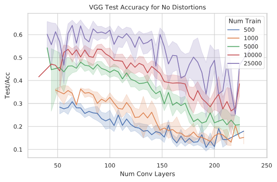
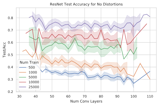
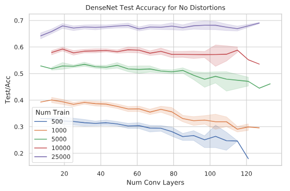
In the default settings we trained the the networks for 100 epochs and randomly sampled ~300 different architectures for each network type (VGG, ResNet, DenseNet). The networks were trained with 500, 1000, 5000, 10k, 25k, and 50k training images from CIFAR10.

The following three graphs show the obtained accuracies for the three architecture types on CIFAR10. Please note, that those accuracies are not necessarily comparable to other papers, as we only trained for 100 epochs due to compute constraints. The three architecture types here are comparable with one another.

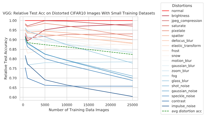
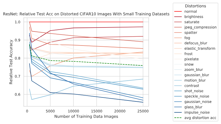
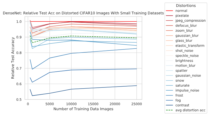
When evaluating the trained models on a distorted CIFAR10 test dataset (15 distortions), we can see that they perform very differently from one another. The three graphs below show the normal distortion (no distortion) as baseline for each number of training samples trained with, and relative to that the performance for distorted test samples. The dashed green line shows the average perfomance of all distortions combined. It is interesting to see, that for VGG and ResNet, distortion robustness on average decreases when trained on more training samples. One issue here could be the CIFAR10 dataset, which is very small and thus distortions might have unpredictable influences on the images at those sizes, making them completely unrecognisable. This is to be investigated further by testing with larger datasets.

DenseNet type networks seem to be significantly more robust against all types of distortions than ResNet and VGG type networks.

Further analysis to come...