Author: Lyuboslav Petrov
This below outlines the work performed for analyzing the German Traffic Sign Benchmark Dataset from the Ruhr-University, Bochum, Germany, as part of the Self Driving Car Engineer nanodegree from Udacity. A convolutional neural network was trained with a validation accuracy of ~94% and testing accuracy of ~95%. Real-world testing with images from the internet showed results approaching 30% accuracy.
One of the main characteristics of a legalized road are its signs and markings. It is therefore of great interest to the self-driving car research domain to find accurate, fast and resilient algorithms for image based road sign detection and classification. This work details the classification aspect, assuming the signs were already detected.
The dataset consists of labeled images organized in train, test and validation sets:
- Number of training examples: 34799
- Number of testing examples: 4410
- Image data shape: 32, 32, 3
- Number of classes: 43
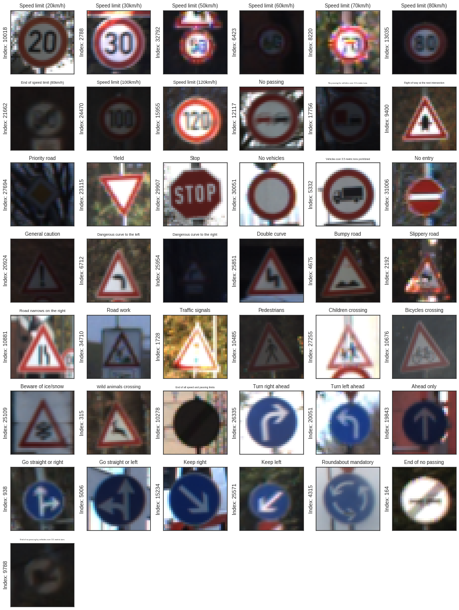
It is evident from the above figure, that there is a great variation of brightness, contrast and resolution in the data. However, the targets/sings are brought to the image foreground and populate the centre of every sample with the majority of pixels, in most cases, belonging to the signs.
The samples per class distribution of all the sets can be seen below:
As can be seen, the distributions along the different sets are very close, but the distribution of samples among classes is of great variance. It was therefore necessary to balance-out the classes by generating surrogate data, based on the existing dataset.
Although the images have already undergone preprocessing steps (ROI cropping), further preprocessing was seen an efficient method for optimizing performance.
Since sample distribution among classes was seen to be greatly varying, it was decided to augment the lower-sample-count classes with artificially created data.
Another benefitial aspect in adding perturbations to the data is that in this manner the network becomes more robust and less likely to overfit.
The methods for creation of this data where all based on perturbing the existing samples, where the perturbations chosen where:
- Image Rotation by +- 6 to 9 degrees around the image centre
- Image Translation by +- 3 pixels along the x and y axes
- Image Affine transformation
- Image Perspective warping
Using these techniques for image generation and class balancing, several balancing thresholds where tested, namely median, mean and max counts of all samples among the classes and the max threshold was chosen as final.
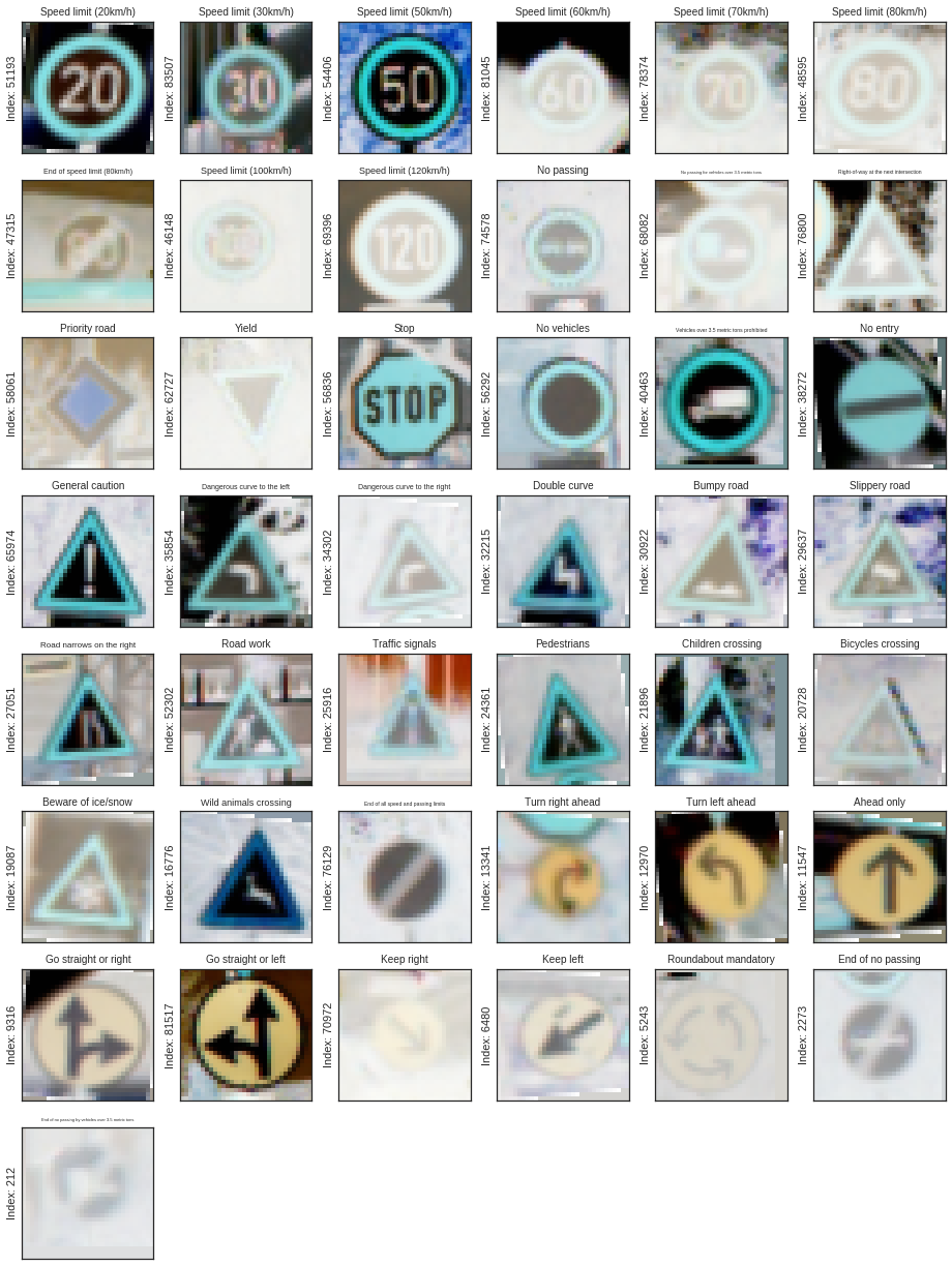
The results from class balancing can be seen below.
NOTE: Images where converted to float32 and therefore their colorspace is depicted differently by matplotlib.
The resulting distribution for the training is shown below, where the total training set size changed from 34799 to 86429, hence the surrogate data represents ~60% of all training data!
Images where then converted to grayscale and normalized between 0 and 1.
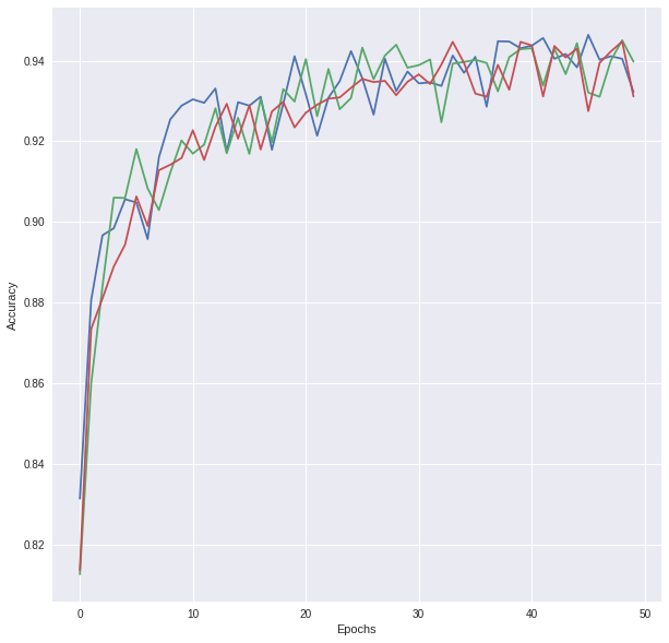
Sevaral network architectures were iterated through. First, the LeNet convolutional network was taken and adapted to work with the traffic sign data set - adapting it to 43 categories, instead of 10. On the first iterations it was observed that the 3 channels of the image do not contribute towards better accuracy and the pre-processing now included not only normalization, but also a colorspace conversion to grayscale. In addition, multiple filter sizes where tested with the LeNet architecture, when the necessity of paramtrization was recognized (see below). Further, two dropout layers were added after the first two Fully-Connected layers which brought the accuracy towards 0.8-0.9. Multiple filter depths were tested, and with filter depths of (64, 128) for the first two convolutional layers, the network reached 0.91 accuracy. A further test was made with addition of a third convolutional layer, where final results came to ~0.95 accuracy.
Details of the layers dimensions can be found below.
In order to iterate through multiple network architectures, it is necessary to make the network models parametric, so interdependencies between variables can be solved dynamically.
Fist, the layer dimensions are sequentially defined. Example:
layers = {}
layers.update({
    'c1':{
        'd': n_channels * 9,
        'fx': 5,
        'fy': 5
    }
})
layers.update({
    'c2':{
        'd': layers['c1']['d'] * 6,
        'fx': 5,
        'fy': 5
    }
})
layers.update({
    'c3':{
        'd': layers['c2']['d'] * 4,
        'fx': 5,
        'fy': 5
    }
})
layers.update({
    'f0': {
        # Resulting flat size = n_channels * 9 * 6 * 4 = 1 * 9 * 6 * 4 = 216
        'in': layers['c3']['d'],
        'out': 480
    }
})
layers.update({
    'f1': {
        'in': layers['f0']['out'],
        'out': 240
    }
})
layers.update({
    'f2': {
        'in': layers['f1']['out'],
        'out': 43
    }
})
Next, the weight and bias objects (python dictionaries) are constructed:
weights = {
    'wc1': tfhe((layers['c1']['fx'], layers['c1']['fy'], n_channels, layers['c1']['d'])),
    'wc2': tfhe((layers['c2']['fx'], layers['c2']['fy'], layers['c1']['d'], layers['c2']['d'])),
    'wc3': tfhe((layers['c3']['fx'], layers['c3']['fy'], layers['c2']['d'], layers['c3']['d'])),
    'wf0': tfhe((layers['f0']['in'], layers['f0']['out'])),
    'wf1': tfhe((layers['f1']['in'], layers['f1']['out'])),
    'wf2': tfhe((layers['f2']['in'], layers['f2']['out']))
}

biases = {
    'bc1': tf.Variable(tf.zeros(layers['c1']['d'])),
    'bc2': tf.Variable(tf.zeros(layers['c2']['d'])),
    'bc3': tf.Variable(tf.zeros(layers['c3']['d'])),
    'bf0': tf.Variable(tf.zeros(layers['f0']['out'])),
    'bf1': tf.Variable(tf.zeros(layers['f1']['out'])),
    'bf2': tf.Variable(tf.zeros(layers['f2']['out']))
}
where, the tfhe function points to the initialization routine detialed in [1].
The initial architecture chosen was LeNet's convolutional network as detailed here. The parameter tweaking and performance testing showed that stacking another convolutional layer is of greater benefit then increasing the number of parameters (i.e. depth vs width).
The final architecture chosen is three subsequent convolutional layers with average pooling, equal strides and equal filter widths (w_c(0,1,2) = 5x5), and respective filter depths (d_c(0,1,2) = 9, 54, 220). The following layers chosen are three subsequent fully connected layers with widths respectively (w_fc(0,1,2) = 480, 240, 43).
| # | Layer | Description | Output |
|---|---|---|---|
| 1 | Input | Grayscale image | 32x32x1 |
| 2 | Convolution (5x5x9) | 1x1 Stride, Valid Padding | 28x28x9 |
| 3 | ReLu | 28x28x9 | |
| 4 | Average pooling | 2x2 stride | 14x14x9 |
| 5 | Convolution (5x5x54) | 1x1 Stride, Valid Padding | 10x10x54 |
| 6 | ReLu | 10x10x54 | |
| 7 | Average pooling | 2x2 stride | 5x5x54 |
| 8 | Convolution (5x5x216) | 1x1 Stride, Valid Padding | 1x1x216 |
| 9 | ReLu | 1x1x216 | |
| 10 | Average pooling | 2x2 stride | 1x1x216 |
| 11 | Fully connected | Flattened network (1x216) | 1x480 |
| 12 | Dropout | val=0.85 | 1x480 |
| 13 | Fully connected | 1x240 | |
| 14 | Dropout | val=0.85 | 1x240 |
| 15 | Fully connected | 1x43 |
The network was trained and optimized for 50 Epochs with a Batch Size of 128 using: For each image, discuss what quality or qualities might be difficult to classify.
| # | Layer | Description | Output |
|---|---|---|---|
| 1 | Softmax | Cross Entropy with Logits | 1x43 |
| 2 | Loss Operation | Reduce entropy with mean | 1x43 |
| 3 | Optimizer | Adam Optimizer (learning_rate = 0.0007) | 1x43 |
The training accuracy achieved was in the range of 0.950-0.960
Testing with images downloaded from a google image search with key-words: "German traffic signs" resulted in accuracy of 0.30.
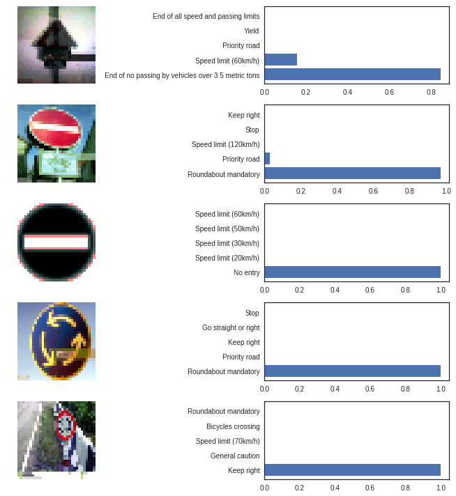
The softmax probabilities 5 randomly chosen real-world images are as follows:
The individual images can below be seen in full size with their supporting discussion.
The top 5 probabilities are far away from correct.
Difficulties for classification:
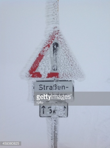
- Snow! This is an image for a General Caution sign in the winter, partially covered in snow.
- Size ratio - the sign area is much smaller than the complete image area (<< 0.5), whereas the training set had a sign to image size ratio of approx 0.5
- Multiple Signs and overlayed text
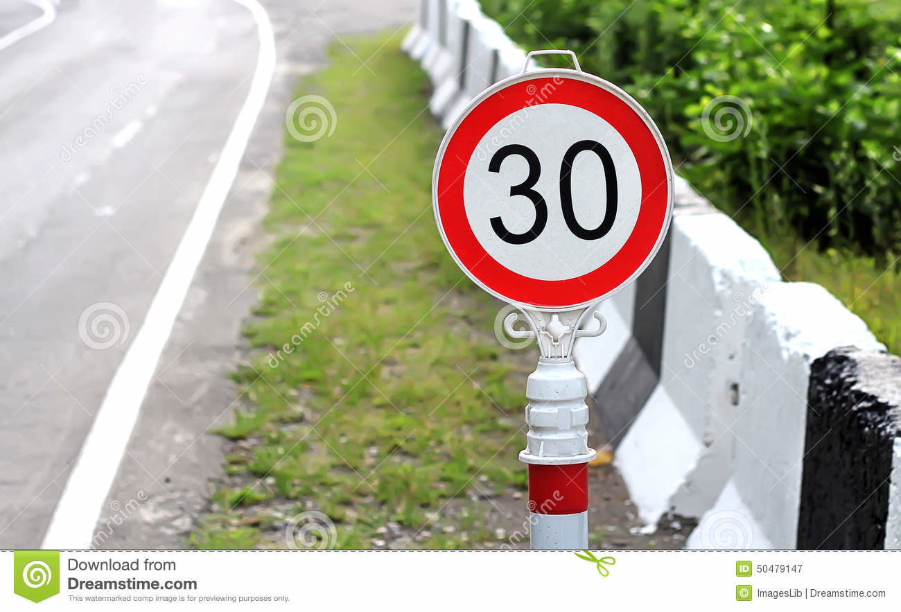
Difficulties for classification:
- Sign centre is shifted towards the upper edge of the image
- The pose of the sign relative to the camera is not favorable to the algorithm
- Size ratio
This image is a drawing and is as expected classified with probability of 1.0
The roundabout mandatory sign is as well classified with a high probability.
Problems with this image are:
- Size ratio (sign area to image area)
The task at hand was successfully completed by achieving a higher than the desired accuracy (testing and validation) of 93%. Further testing with random images from the internet showed the weakness of the model, namly that it expects the sign to be centrally located within the image, to be of a certain resolution and to occupy the bulk are within the image. Prior data augmenting, real-world results were with accuracy < 0.1. After augmentation, the results improved significantly.
During training and testing it was noted that increasing the dropout rate above 0.5 up to 0.9 had only benefitial effects. This can be attributed to the intentionally wide fully connected layers at the end, where a large dropout will still result in enough nodes left to achieve a good result.
The conversion to grayscale proved itself also very valuable. This operation is essentially a pre-convolution that reduces the dimensionality of the input set, which in turn reduces drastically the requirements for the network size with negligable information loss.
Increasing network depth was the final step following which the desired accuracy was exceeded.
N/A
[1] Kaiming He, Xiangyu Zhang, Shaoqing Ren, Jian Sun, "Delving Deep into Rectifiers: Surpassing Human-Level Performance on ImageNet Classification", CoRR, 2015
