AccidentAnalysis: A Jupyter Notebook repository from nirajsaran2

Sober Truths

EDA: Looked at the large number of pre-crash conditions, road surface conditions, driver distractions including by a mobile device or texting, vision obscured by rain/snow, construction zone, maneuvering to avoid another vehicle or pedestrians or bicyclists, contributing factors like tires, brakes or headlights, bad weather or poor lighting conditions, among others. Also looked at state, city and lat/long data. This is a very rich set of data and there is literally no limit to the amount of Eda once can do.

For the time series model, I was able to use the NHTSA accident dataset directly since this has all the drunk driver, pedestrians, vehicle and persons information aggregated for a crash. Creating a datetime index, resampling by day, week and month generated the dataframes necessary for modeling by day, week and month respectively.

3 Hour window:

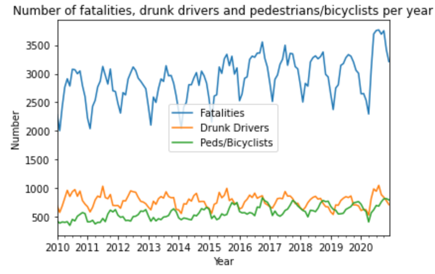
Looking at visualizations by year, month, week, day of week or hour of day did not give too many insights other than the trend of fatalities, drinking drivers and pedestrians killed has been mostly increasing over the years.

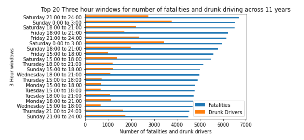
A key discovery from the EDA and external research was that weekend nights have more accidents and a larger percentage are caused by drinking drivers. This led to creating shorter periods of 2, 3 and 4 hours to determine patterns. This was huge

This led me to dive a lot deeper into the dataset using this 3 hour window to determine the causes and potential ways to reduce the fatalities during the worst times.

Details in subsequent sections.

Model Selection:

The dataset contains sequential temporal data and is hence a good candidate for time series based models.

The two most popular models for time series forecasting are AutoRegressive and RNN.

Among AutoRregressive options like ARIMA, SARIMAX etc, I chose the Vector AutoRegressive (VAR) model since it is a bi-directional multivariate forecasting algorithm where two or more time series influence each other. In our case, the number of fatalities, alcohol-impaired drivers, pedestrians killed, vehicles and persons involved influence each other. Each of these variables is modeled as a linear combination of past values of itself (lags) and the past values of these other variables.

Used correlation to confirm that these influence each other and hence can use the VAR model to forecast all five variables.

Did the diff and used the ADF (Augmented Dickey Fuller) statistical Test to confirm stationarity of the time series variables.

The coefficient of correlation between two values in a time series, called the autocorrelation function (ACF) was used to identify seasonality in our time series data.

The ACF plot, a bar chart of the coefficients of correlation between a time series and lags of itself, was used to pick the points that are statistically significant (outside the blue shaded Confidence Interval region).

Partial autocorrelation (PACF), a statistical measure that captures the correlation between two variables after controlling for the effects of other variables, was used to confirm the statistically significant lags.

We then decomposed the three parts of a time series – the trend, seasonality and residuals for all 5 variables.

Then came the traditional instantiate, fit, predict and evaluate.

Recurrent Neural Networks are deep learning models used to solve problems with sequential input data. I used the same five variables in the RNN model, as all the inputs are related to one another, to enable easier comparison between the two models.

Similar to linear regression models, and unlike the time series, these variables are like the X variables used for predictions and the target variable is just the fatals.

I used a small test size of 2% during the train test split and the Keras TimeseriesGenerator to feed 16 sequences (batchsize) of length of 3 (and 5) through our model. Our validation data set is small (only 81 rows) so chose a small batch size of 16. The length is the number of lag observations to be used in the input portion of each sample.

LSTM (long short-term memory) and GRU (Gated Recurrent Units) can alleviate the vanishing gradient problem which is a known shortcoming of RNNS especially with long time series extending over hundreds of periods. Along with Regularization using Dropout layers and EarlyStopping for optimization, I was able to get to a reasonably performing predictive model.

Model Evaluation:

Used RMSE and MAPE to see how far off are predictions are in absolute numbers (in the same units as our target) and in percent terms.

Findings and Observations

EDA:

Started with 356445 records for 11 years, after cleanup 353764.

Interpretation:

The largest number of alcohol-impaired driver (AID) involved fatal crashes is Sunday midnight to 3am i.e. late Saturday night, followed by Saturday midnight to 3am, i.e. late Friday night.

Interpretation:

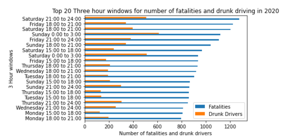
In 2020, 55% of fatalities were caused by drinking drivers during the worst 3 hour window of Sunday midnight to 3am.

Overall across all 11 years, it was 57%.

In 2020, there were 38491 fatalities. Average of 105 per day, or 4.4 per hour

During the worst 3 hour window of Saturday 21:00 to 24:00, there were a total of 1273 fatalities in 2020, average of 24.5 per week per this 3 hour window, i.e. 8.1 per hour. During Labor Day, it went up to 11 per hour.

This is 2.5 times the hourly average of 4.4.

In 2020, there were 9415 drinking driver fatalities. Average of 25.8 per day, or 1.1 per hour

During the worst 3 hour window of Sunday 0:00 to 3:00, there were a total of 610 drinking driver fatalities in 2020, average of 11.7 per week per this 3 hour window, i.e. 3.9 per hour. During Labor Day, it went up to 5.6 per hour.

This is 3.5 times the hourly average of 1.1

Percent:

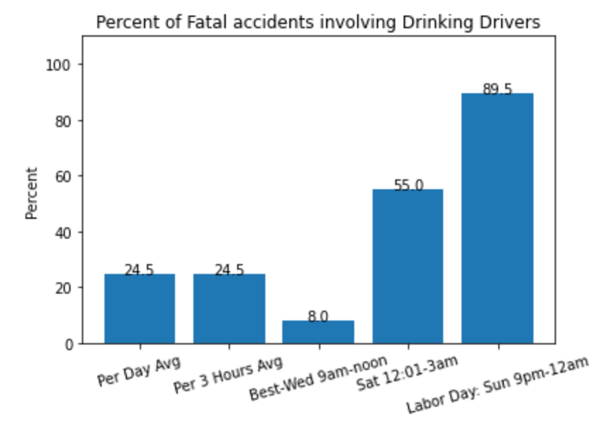
In 2020, 24.5% of fatalities (9415 out of 38491) involved drinking drivers. During weekend nights, this percent went up to 55%. During Labor Day, it went up to 89.5%

Interpretation: 57% of all fatalities are caused by drinking drivers on Saturday and Friday nights.

Only 7% of fatalities are caused by drinking drivers on Wednesday and Thursday from 9am-noon.

Holidays:

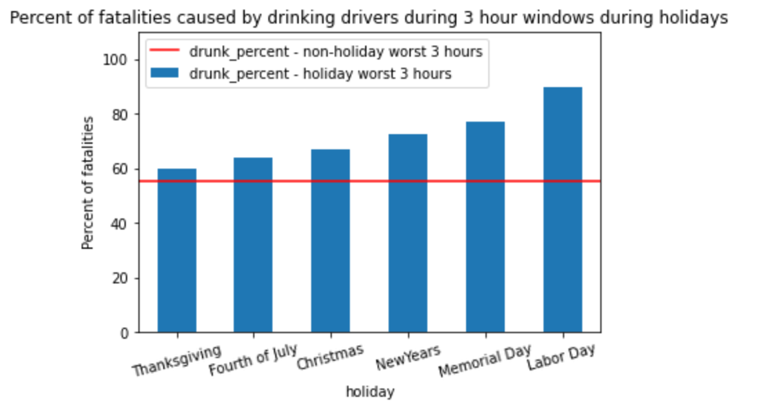
Another key finding was that during the major holidays – Labor Day, Memorial Day, New Year’s Day the percent of AID involvement shot up to as much as 90%

Interpretation:

During Holidays, there are many more fatalities caused by drinking drivers than during the worst 3 hour windows on non-holidays.

During the Labor Day weekend, 90% of the 19 fatalities were caused by drinking drivers on Sun between midnight and 3am, and 75% of the 20 fatalities on Sat between midnight and 3am. Both these percentages are well above the 55% of drinking driver fatalities on non-holiday weekends.

In 2020, of the total 9415 drinking driver fatalities, 803 (8.5%) were during the 6 holidays. Fatalities were 2412 (6.3%) during the Holidays

	Total in 2020	Per Day Avg	Per 3 Hours Avg	Late Sat: Sun 12:01-3am hours	Labor Day: Sun 9pm-midnight	Lowest-Wed 9am-noon
Fatalities	38491	105.5	13.2	24.5	33.0
Drunk Drivers	9415	25.8	3.2	11.7	17.0
Percent Drunk Drivers	24.5	24.5	24.5	55.0	89.5	8.0

On average, 24.5% of fatalities involve drinking drivers. During the best 3 hour window, on Wednesdays between 9am and noon, only 8% of fatalities are caused by Drinking Drivers.

However, during the worst 3 hour window which is late Saturday night - i.e. Sunday 12:00am-3am, the percentage goes up to 55% and even worse is on Holidays like Labor Day when the percentage is 89.5%.

The range is from 8% to 90% - this clearly calls for better sobriety checks and roving patrols during the hours from 9pm to 3am on Holidays and weekends.

VAR Modeling Findings:

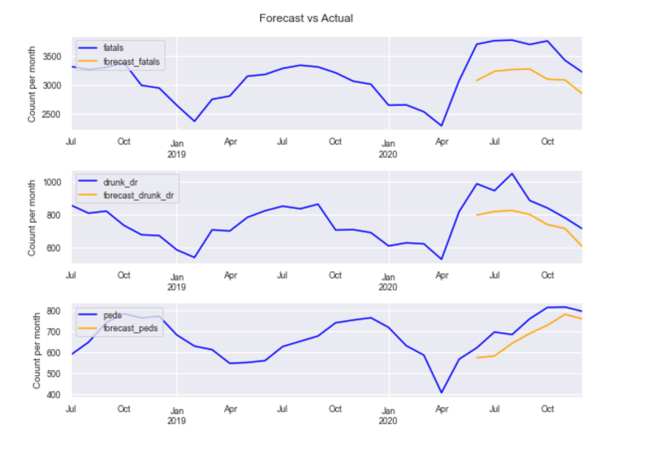
Used a Train Test Split of 5% since forecasting works better for small time periods and our monthly time series for 11 years has only 132 data points. Using maxlags during fitting, the order of the timeseries (number of lags used in the model) is 13. There are no other hyper-parameters to tune, except to ensure that the time series is stationary.

Monthly – needed one diff to make stationary. Weekly and daily were already stationary.

Interpretation:

The forecast does a pretty good job in following the actual curve except where the data spikes suddenly.

Model Evaluation:

The test RMSE is substantially better than the baseline RMSE, for all 3 variables. For fatals, the test RMSE of 503 is 34% better than the baseline of 761.9.

The Mean Absolute Percent Error (MAPE) which shows the percent error indicates that our model’s forecast for fatals is off by 14% on an average month or 503.

The forecast for the peds is the most accurate, its off by 8% or 67 peds per month, in an average month.

RNN:

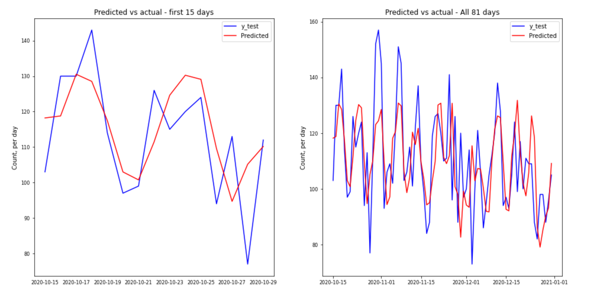
The daily time periods spanning 11 years has a total of 4018 observations, of which the validation data of 2% is 81 observations.

Tried various models with varying sequence of length size and LSTM and GRU layer with regularization, different number of hidden layers and nodes and Dropout.

The params for the best model are in a later section.

Interpretation:

The predictions are quite good, more so in the first few days. Over the total 81 days of predictions, the predictions don't quite match the peaks. In fact, towards the end they overshoot the data considerably.

Interpretation:

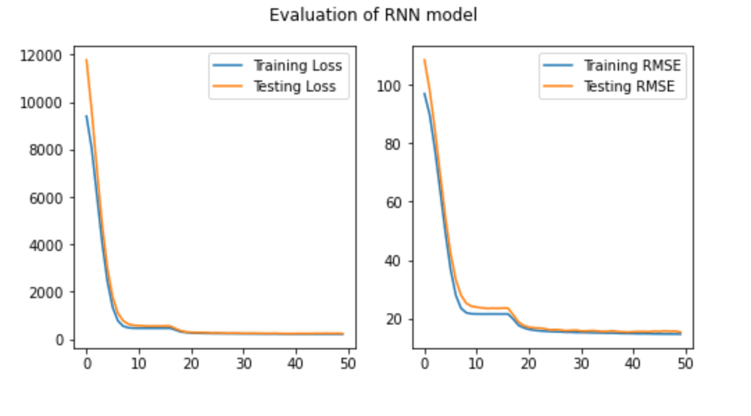
The graphs are almost perfect! The testing RMSE is marginally higher than the Training RMSE, showing the model is not overfit and should do a good job on predicting new unseen data.

Model Evaluation:

Baseline RMSE	Training RMSE	Test RMSE	Baseline MAPE	Training MAPE	Test MAPE
23.25	14.69	15.32	0.15	0.12	0.10

The RMSE and MAPE confirm the graphs. The Training RMSE is substantially better than baseline and the Test RMSE is only marginally higher than the Training RMSE.

This indicates that our model’s forecast for fatalities is off by 10% on an average day or 15.

Conclusions

VAR: Testing RMSE: 503/30=16, Testing MAPE: Fatals: 0.14, Peds: 0.08

RNN: Testing RMSE: 15.32, Testing MAPE Fatals: 0.10

Both did quite well, though RNN is lightly better on fatalities.

VAR gets to forecast on more than one variable and did a really good on forecasting pedestrian fatalities.

Best Params:

RNN:

2 GRU hidden layers of 16 and 8 nodes

Dense hidden layer with 8 nodes

Output layer (1 node, regression, relu activation)

Next Steps

Need to tune the models to improve performance (time consuming and CPU intensive)
Room for improvement:
- Try Linear Regression with exogenous variables – weather, distracted, construction zone
- VAR: investigate how to improve weekly and daily forecasts
- RNN: Can try weekly and monthly resampling to compare with VAR. Could try further hyper-parameter tuning
- Clean up warnings

Bibliography

Fatality Analysis Reporting System (FARS) Analytical User’s Manual, 1975-2020: https://crashstats.nhtsa.dot.gov/Api/Public/ViewPublication/813254
Fatalities and Coding and Validation manual: https://crashstats.nhtsa.dot.gov/Api/Public/ViewPublication/813251

nirajsaran2/AccidentAnalysis

Sober Truths

Contents:

Problem Statement

Summary

Data Dictionary

Input Data

Output Data files

Image files

Methodology

Findings and Observations

Conclusions

Next Steps

Bibliography