Git page for stockassessment R-package containing the state-space assessment model (SAM)
Can be installed by typing:
devtools::install_github("fishfollower/SAM/stockassessment")(To ensure only installing in 64-bit some windows users may need to install with:
devtools::install_github("fishfollower/SAM/stockassessment",
                          INSTALL_opts=c("--no-multiarch"))
)
Alternatively it can be installed from r-universe by:
install.packages('stockassessment',
                 repos=c(CRAN="https://cloud.r-project.org/",
SAM='https://fishfollower.r-universe.dev'))We start by downloading a few needed files. Here the files are taken from one of the test cases (North Sea Herring). We use a temporary folder to make sure we are not overwriting existing files.
setwd(tempdir())
filestoget <- c("cn.dat", "cw.dat", "dw.dat", "lf.dat", "lw.dat",
                "mo.dat", "nm.dat", "pf.dat", "pm.dat", "sw.dat",
                "survey.dat")
url <- "https://raw.githubusercontent.com/fishfollower/SAM/master/stockassessment/tests/nsher/"
d <- lapply(filestoget, function(f)download.file(paste(url,f,sep=""), f))
Now the files should be downloaded to our current working directory. Next we read in the data files and create a collected data object:
library(stockassessment)
cn <- read.ices("cn.dat")
cw <- read.ices("cw.dat")
dw <- read.ices("dw.dat")
lf <- read.ices("lf.dat")
lw <- read.ices("lw.dat")
mo <- read.ices("mo.dat")
nm <- read.ices("nm.dat")
pf <- read.ices("pf.dat")
pm <- read.ices("pm.dat")
sw <- read.ices("sw.dat")
surveys <- read.ices("survey.dat")

dat <- setup.sam.data(surveys=surveys,
                      residual.fleet=cn,
                      prop.mature=mo,
                      stock.mean.weight=sw,
                      catch.mean.weight=cw,
                      dis.mean.weight=dw,
                      land.mean.weight=lw,
                      prop.f=pf,
                      prop.m=pm,
                      natural.mortality=nm,
                      land.frac=lf)
From this defined data object it is possible to generate a default/minimalistic model configuration.
conf <- defcon(dat)This configuration can be changed by modifying/overwriting the elements in the list. Here we set the fbar range to 2-6, allow correlated F processes, and modify the catchability couplings.
conf$fbarRange <- c(2,6)
conf$corFlag <- 1
conf$keyLogFpar <- matrix(c(
-1,   -1,   -1,   -1,   -1,   -1,   -1,   -1,   -1,
-1,    0,    1,    2,    3,    4,    5,    6,   -1,
-1,    7,   -1,   -1,   -1,   -1,   -1,   -1,   -1,
 8,   -1,   -1,   -1,   -1,   -1,   -1,   -1,   -1), nrow=4, byrow=TRUE)
Now the configuration and data is in place, so we can generate default initial values for all our model parameters.
par <- defpar(dat,conf)These default initial can be modified (like the configuration), but it is rarely necessary. To illustrate we modify the initial values for the catchabilities
par$logFpar <- rep(0,9)Now we are ready to optimize the model.
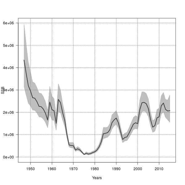
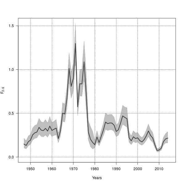
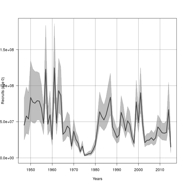
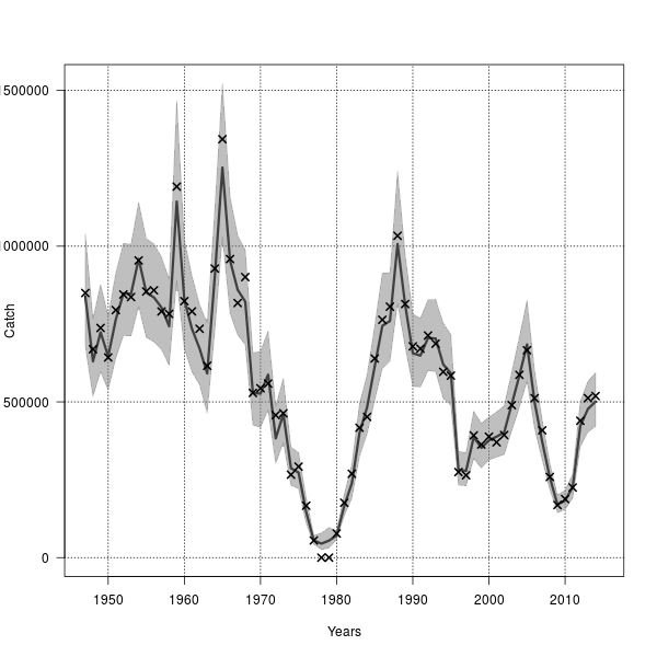
fit <- sam.fit(dat,conf,par) This fitted model object contains all information about the fit and can be used to plot and extract all requested quantities. Let's plot the SSB, Fbar, rectuitment, and total catch.
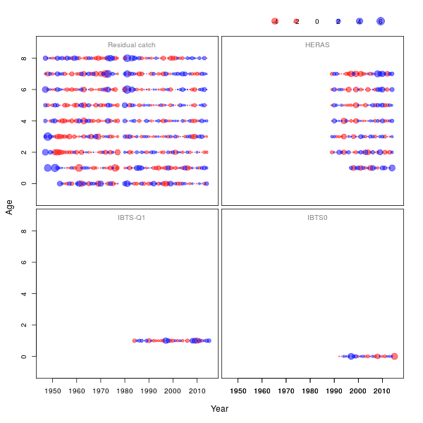
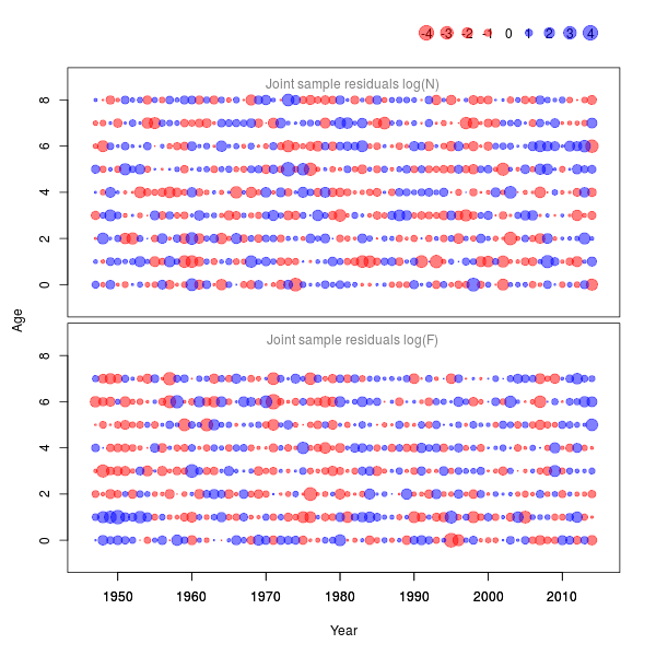
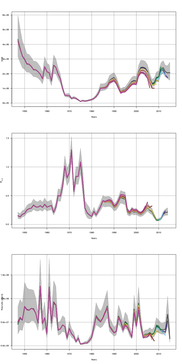
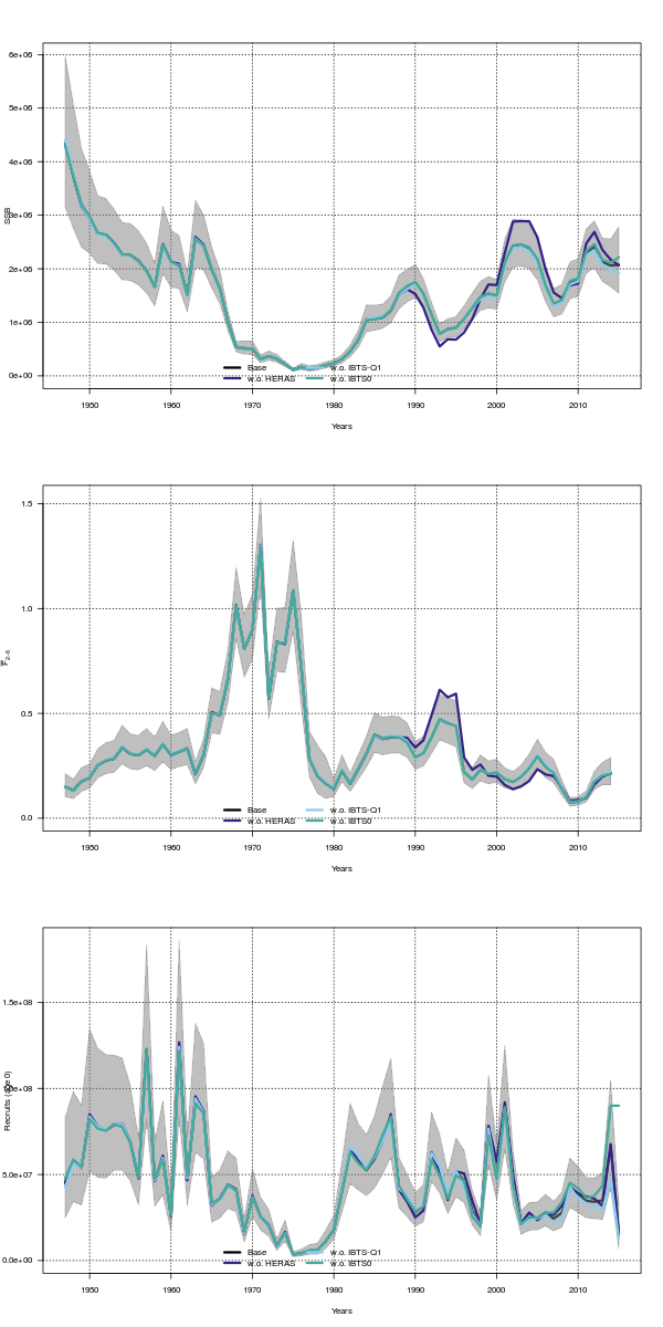
ssbplot(fit)fbarplot(fit)recplot(fit)catchplot(fit)Model diagnosis in terms of residuals (one observation ahead residuals, and process joint sample residuals), retrospective, and leave-out can be computed and plottet in the following way.
res <- residuals(fit)
plot(res)
resp <- procres(fit)
plot(resp)retro <- retro(fit,year=10)
plot(retro)lo <- leaveout(fit)
plot(lo)