Introduction to PAC Learning Theory

Introduction

Probably Approximately Correct (PAC) computational learning theory provides a mathematically rigorous definition of what machine learning is.

So far, we have looked into steps required in order to run machine learning algorithms including data representations, feature selection and engineering, training, prediction and evaluation of results. In this lesson, we shall provide a brief overview of a Probably Approximately Correct or PAC learning theory that provides a foundation for experimental settings that we have looked at so far. In essence , PAC deals with the computational aspect of machine learning. The theory helps us deal with sample complexity and associated computational complexity in order to answer an analytical question.

Objectives

You will be able to:

Understand and describe the PAC learning theory
State how PAC theory relates to computational (machine) learning practices
Identify the major factors of PAC theory and describe how the error and confidence measures are used to approximate a desired function

Intuition behind PAC

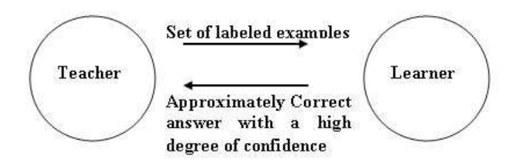
The PAC is a learning models which is characterized by learning from examples.

In its simplest form, consider $f$ as the target function to be learnt, the learner (the computational model) is provided with some random examples in the form of $(X,f(X))$.

Here, $X$ is a binary input instance of length $n$, and $f(X)$ is the value (boolean TRUE or FALSE) of the target function at that instance.

Based on these examples, the learner must succeed in deducing the target function $f$ which is expressed as:

$$f : [0, 1]^n → {0, 1}$$.

What do we actually mean by success? It should actually be any measure or a series of evaluation steps that help us find that the algorithm meets the criteria. Hence this approach can b shown using the model below:

Failure Probability

According to PAC, there is always a small probability that the learning algorithm fails and the results produced are not accurate. One obvious reason could be that learning examples do not fully reflect the probability distribution that the examples belong to, and. i.e. This hinders l learning process seriously and target function $f$ can not be achieved. insufficient examples is something that we come across very often in machine learning discipline. PAC Learning attempts to reduce the probability of getting such poor examples by considering a sufficient number of examples for learning the required function.

PAC learning approach places an upper bound on the probability of error by placing a lower bound on the number of examples required to learn the target function.

Function Approximation

In PAC, we do not expect the learner to learn the exact function most of the time, due to limits on available examples and noise in the data etc. We expect the learner to find a function $h$ which is very close to the desired function $f$. So we say that $h$ approximates $f$ , and that is function we are interested in learning.

The two factors given above are to explain the meaning of success.

"Probably: " If learner outputs the data with desired probability and confidence, the results are probably correct

"Approximately: ." A hypothesis is approximately correct if its error over the distribution of inputs is bounded by some predefined interval.

The results of PAC learning are therefore called "Probably Approximately Correct"

Error Calculation

Based on these, PAC gives:

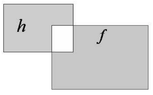
an upper bound on the error in accuracy with which h approximates f and
the probability of failure in achieving this accuracy.

With these quantities, we an express the definition of a PAC Algorithm with more mathematical clarity.

For PAC Learnability, the learner must find a concept $h$ such that the error between $h$ and $f$ with acceptable range with a predefined level of confidence.

The notion of approximation is described as: There is some probability distribution $D$, defined in the sample sample $[0,1]|^n$ giving probability of each example. So we are picking examples from this distribution, at random. Also, its imperative to mention that the all the examples that learner is provided with are iid ,independent and identical . Considering the total probability of seeing a sequence of examples over $D$ , we will use the product rule.

The distribution $D$, conveniently and mathematically quantifies the error with which $h$ approximates $f$ as shown below:

$$err(h, f) ≡ P_{x∈D}(h(x) \neq f(x))$$

$P_{x∈D}$ reflects the probabilities are taken with respect to random draws over $D$ only. In terms of set theory, our error is the symmetric difference between the sets corresponding to $h$ and $f$ over $X$, shown in the shaded areas below, highlighting probabilistic region of disagreement between $h$ and $f$ and hence gives the probability of error:

A PAC Learning Algorithm would always be independent of underlying distribution i.e. $D$. The only restriction on the setting is that we must calculate the probability of error over the same distribution from which we draw our iid examples. The learner sees examples so that the probability of a poor example i.e. an error over the same distribution reduces to some specified bounds. It is therefore natural to calculate the error probability over the same distribution that was used during the learning phase. And as you can see, we have taken care of this fact in equation above which calculates the probability over D only.

PAC Examples

Visit this link for detailed problem definitions with mathematical proofs and intuitions behind some PAC theorems. The document entails following problems that a PAC learnable.

Learning positive half-lines
Learning intervals
Learning axis-aligned rectangles

How PAC relates to Machine Learning

PAC uses the term 'hypothesis',whereas ML literature normally uses the term 'model'. So we have seen that Machine learning starts with some data, (xi,yi) and we want to find a hypothesis (or model) that will, given the inputs xi return yi or something very close. More importantly given new data x̃ the model will predict the corresponding ỹ.

A model that was created using some (out of many examples) of data do not accurately reflect that data set, but can be accurate on any future data sets. The two important points are that we cannot predict new data with 100% accuracy. There is also the possibility that the one or more examples are poor and do not explain much.

We present our data to the learner and let it make an attempt to learn the hypothesis function. At discrete stages ,we then look at the error as the difference between real and hypothesis function outputs. A problem is called learnable if we can reduce this error within acceptable bounds.

SO that is PAC. It is essentially provides theoretical and mathematical underpinning to different stages of machine learning that we have been looking at in our course. This theory justifies the need for splitting data into test and training sets. It gives a reason to tune hyper parameters as the learner is independent of the data distribution. This theory also provides grounds for the evaluation methods we have seen including RMSE, ROC, AUC etc. to ensure that our model is learning and approximating a desired function.

Additional Resources

A deeper understanding of PAC requires looking at some examples with proofs of how we identify PAC learnability. You are encouraged to visit following resources which will elaborate the points highlighted in this lesson.

Summary

In this lesson, we looked at how PAC learning allows us to develop models , train and evaluate them in a computational learning domain. We looked at developing a basic intuition behind this theory and how it relates to different stages of model development that we have been looking at. You are encouraged to read into this theory and try to relate all the upcoming architectures to this theory to help you develop a sound and scalable understanding of ML from theory to practice.

nitdip/dsc-3-31-02-introduction-to-PAC-learning-theory-online-ds-pt-100118