Welcome to NumbaSOM

A fast Self-Organizing Map Python library implemented in Numba.

This is a fast and simple to use SOM library. It utilizes online training (one data point at the time) rather than batch training. The implemented topologies are a simple 2D lattice or a torus.

How to Install

To install this package with pip run:

pip install numbasom

To install this package with conda run:

conda install -c mnikola numbasom

How to use

To import the library you can safely use:

from numbasom import *

A Self-Organizing Map is often used to show the underlying structure in data. To show how to use the library, we will train it on 200 random 3-dimensional vectors (so we can render them as colors):

Create 200 random colors

import numpy as np
data = np.random.random([200,3])

Initialize the library

We initalize a map with 50 rows and 100 columns. The default topology is a 2D lattice. We can also train it on a torus by setting is_torus=True

som = SOM(som_size=(50,100), is_torus=False)

Train the SOM

We will adapt the lattice by iterating 10.000 times through our data points. If we set normalize=True, data will be normalized before training.

lattice = som.train(data, num_iterations=15000)

SOM training took: 0.366633 seconds.

To access an individual cell type

lattice[5,3]

array([0.92550425, 0.20740594, 0.92610555])

To access multiple cells, slicing works

lattice[1::6,1]

array([[0.7473038 , 0.09876245, 0.93051731],
       [0.93542156, 0.18717452, 0.87611239],
       [0.9486485 , 0.11080808, 0.57557379],
       [0.87873391, 0.13527156, 0.368202  ],
       [0.78669284, 0.11830203, 0.2634972 ],
       [0.68213238, 0.06408478, 0.33050376],
       [0.54769163, 0.05391318, 0.31153485],
       [0.63722088, 0.12484291, 0.0684501 ],
       [0.64172725, 0.01517416, 0.09549566]])

The shape of the lattice should be (50, 100, 3)

lattice.shape

(50, 100, 3)

Visualizing the lattice

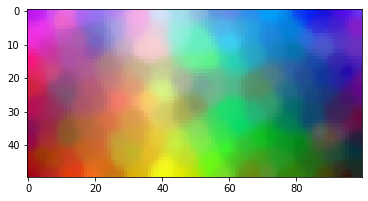
Since our lattice is made of 3-dimensional vectors, we can represent it as a lattice of colors.

import matplotlib.pyplot as plt

plt.imshow(lattice)
plt.show()

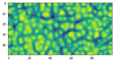
Compute U-matrix

Since the most of the data will not be 3-dimensional, we can use the u_matrix (unified distance matrix by Alfred Ultsch) to visualise the map and the clusters emerging on it.

um = u_matrix(lattice)

Each cell of the lattice is just a single value, thus the shape is:

um.shape

(50, 100)

Plot U-matrix

The library contains a function plot_u_matrix that can help visualise it.

plot_u_matrix(um, fig_size=(6.2,6.2))

Project on the lattice

To project data on the lattice, use project_on_lattice function.

Let's project a couple of predefined color on the trained lattice and see in which cells they will end up:

colors = np.array([[1.,0.,0.],[0.,1.,0.],[0.,0.,1.],[1.,1.,0.],[0.,1.,1.],[1.,0.,1.],[0.,0.,0.],[1.,1.,1.]])
color_labels = ['red', 'green', 'blue', 'yellow', 'cyan', 'purple','black', 'white']

projection = project_on_lattice(colors, lattice, additional_list=color_labels)

for p in projection:
    if projection[p]:
        print (p, projection[p][0])

Projecting on SOM took: 0.158945 seconds.
(0, 85) blue
(2, 39) white
(5, 1) purple
(10, 60) cyan
(41, 59) green
(49, 12) red
(49, 40) yellow
(49, 96) black

Find every cell's closest vector in the data

To find every cell's closes vector in the provided data, use lattice_closest_vectors function.

We can again use the colors example:

closest = lattice_closest_vectors(colors, lattice, additional_list=color_labels)

Finding closest data points took: 0.003056 seconds.

We can ask now to which value in color_labels are out lattice cells closest to:

closest[(1,1)]

['purple']

closest[(40,80)]

['green']

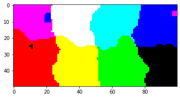
We can find the closest vectors without supplying an additional list. Then we get the association between the lattice and the data vectors that we can display as colors.

closest_vec = lattice_closest_vectors(colors, lattice)

Finding closest data points took: 0.003491 seconds.

We take the values of the closest_vec vector and reshape it into a numpy vector values.

values = np.array(list(closest_vec.values())).reshape(50,100,-1)

We can now visualise the projection of our 8 hard-coded colors onto the lattice:

plt.imshow(values)
plt.show()

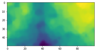
Compute how each data vector 'activates' the lattice

We can use the function lattice_activations:

activations = lattice_activations(colors, lattice)

Computing SOM activations took: 0.000484 seconds.

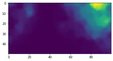
Now we can show how the vector blue: [0.,0.,1.] activates the lattice:

plt.imshow(activations[2])
plt.show()

If we wish to scale the higher values up, and scale down the lower values, we can use the argument exponent when computing the activations:

activations = lattice_activations(colors, lattice, exponent=8)

Computing SOM activations took: 0.000838 seconds.

plt.imshow(activations[2])
plt.show()

nmarincic/numbasom