This analysis shows an application of Principal Component Analysis in order to develop a pairs trading strategy to capture statistical arbitrage in the Precious Metals Market.
We are going to look at how using PCA to create "eigenportfolios" that can be used to obtain a Sharpe Ratio of 1.093 and a Sortino Ratio of 1.578 using a risk-free rate of 2%.
This dataset deals with the london fix spot prices for gold, silver, platinum, and palladium. It was taken from: https://www.perthmint.com/historical_metal_prices.aspx
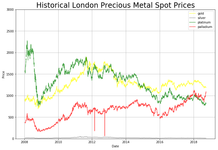
In this analysis, we used the price data for the past 10 years, from 2008 - 2018. The london fix has an AM and PM fix for gold, platinum, and palladium, while it only has 1 fix for silver.
Since we need to treat the AM and PM fix as different events, we separate this so that each fix represents a row in the dataset. Since Silver only has one fix, we will duplicate its fix price for both the AM and PM value.
Notice the drastic spikes in Palladium in 2012. We think this is due to some documentation error or some fluke, so we will exclude these values from our dataset.
We are now going to use PCA (Principal Component Analysis) in order to decompose this historical market. PCA is a popular technique used in data science to reduce the dimensionality of the data while retaining as much information of the data as possible.
We now perform Singular Value Decomposition of the Covariance Matrix.
Where the  corresponds to the Left Principal Components,
  corresponds to the diagonlized Eigenvalues in ascending order, and
  corresponds to the Right Principal Components.
Theoretically, PCA tries to project a  -dimensional space into a smaller
  -dimensionsal space, where
  >>
>>  .
.
It does this by decomposing the co-variance matrix,  which is the matrix of datapoints
whose
  th element is the covariance between the
  th and
  th element in a random vector.
The principal components of the decomposition of the covariance matrix that capture the most information of the dataset whenever the dataset is projected onto that vector. The Eigenvalue that corresponds to that eigenvector is how strongly that eigenvector explains the variance of the data. The left singular vectors tell us how much each particular row accounts for the variance of the data, while the right singular vectors tell us how much each particular column to the data.
Following from our knowledge of what PCA does fundamentally to an arbitrary dataset, how can we interpret it when applied to trading data?
Suppose we have a matrix  that represents a basket of
  stocks over
  days. Whenever we take take the Principal Component Analysis of this matrix, we are left with a decomposition of the left principal
components multiplied by the eigenvales multiplied by the right principal vectors.
The eigenvalues represent how much of the variance of the dataset is captured in each "concept" of the dataset.
The left eigenvectors can be interpreted as how much the rows (a.k.a the stocks) correspond to each concept.
The right eigenvectors can be interpreted as how much the columns (a.k.a the daily prices) correspond to each concept.
After decomposing the Covariance Matrix of our metal prices, we are left with the following interpretation:
Each eigenvalue corresponds to the how much of the total variance of the data the corresponding principal component captures.
The corresponding principal component represents a portfolio allocation that captures that amount of variance.
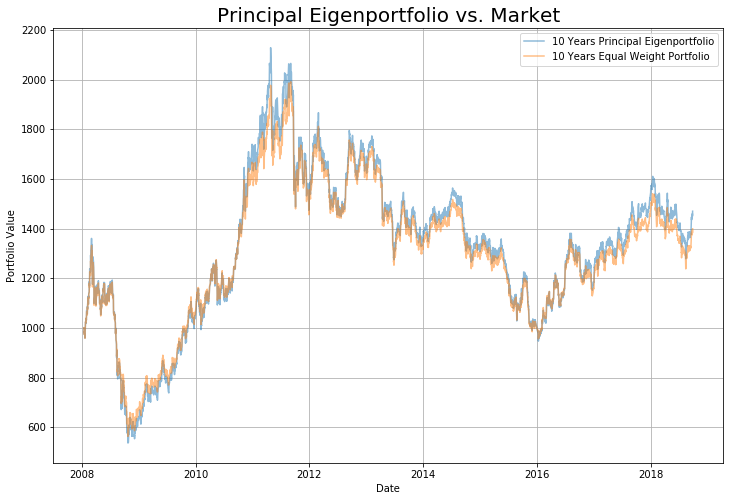
It can be seen from the image above that the eigenvector portfolio allocation that captures the most variance (a.k.a. the top eigenvector) is almost identical to the market.
This phenomenon is due to Krein's Theorem.
When all assets have non-negative correlation, the coefficients of the first principal component are all non-negative.
We already know that each principal component represents a portfolio allocation. Now that we are guaranteed that the first principal component has all non-negative coefficients, we can interpret the first principal component as the vector that characterizes "market forces", since it takes a long position in every underlying.
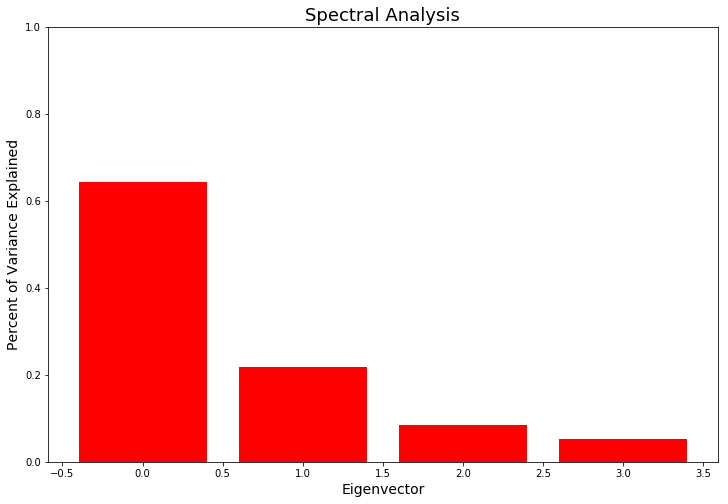
The corresponding eigenvalue shows how much of the total variance of the data is explained by market forces.
The graph above shows the spectral analysis of the principal components. It can be seen that the principal eigenvector or "market vector" captures around 65% of the variance explained in the data. The other eigenvectors capture the intercompany variance and noise.
It follows that all other eigenportfolios of the eigenbasis is orthogonal to the first principal component. This means that it's "uncorrelated" with the market, and hence, market neutral.
Furthermore, since the principal component has all positive coefficients, the orthogonal eigenvectors must have at least 1 negative coefficient.
Therefore, we claim that the orthogonal eigenvectors represent a market neutral pairs trading strategy that aims to capture the variance not explained by the market.
In the next section, we show that utilizing the orthogonal vectors as a market neutral pairs trading porfolio leads to promising profits.
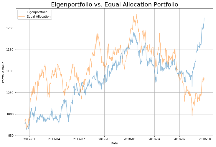
We will now try to backtest this algorithm by training on the first 8 years of historical data and then testing it on the final 2 years.
The second eigenportfolio allocation performs well, capturing the variance of historical returns between precious metals and earning a respectable 25% return over 2 years.
The portfolio allocation used was as follows: [Gold, Silver, Platinum, Palladium] [-0.10754848 -0.67890968 0.19386913 0.69994981]
The eigenportfolio technique is an interesting way to decompose a sector and potentially find market neutral pairs trading opportunities between different assets of a sector.
Given the right circumstances, we can use it to obtain a respectable profit of 25% over 2 years in the precious metals market, as shown in backtesting.
Below are some of the caveats and next steps for this project.
-
Volatility effects the eigenportfolios by a lot. We need to explore the effects of normalizing by volatility.
-
This assumes the market forces are linear. Will need to investigate results by using non-linear PCA.
-
This is constrained to groups of assets where all assets are correlated with each other to some degree.
-
Will need to look at backtesting results when eigenportfolios are dynamically rebalanced.
-
look at very stable markets, medical equipment, construction, retail, semiconductor, things that are robust to policy related volatility


