Implementation of Numerical Gaussian Processes in C++
- Eigen - High-level C++ library for linear algebra, matrix operations, and solvers (version 3.3.7)
- GCC - GNU compiler collection; more specifically the GCC C++ compiler is recommended
- LBFGS++ - A header-only implementation of the L-BFGS algorithm in C++
- NumPy - Scientific computing package for Python
- csv - Python module for working with comma separated value (csv) files
- MatPlotLib - Python plotting library
- SciKit Learn - Data analysis library for Python
- PyTorch - Open source deep learning platform
- GPyTorch - PyTorch implementation of Gaussian processes with extensive modeling capabilities
The main.cpp file provides an example use of the CppGP code for Gaussian process regression. Before compilation, the following steps must be carried out:
- Specify the path to the Eigen header files by editing the
EIGENPATHvariable inmakefile - Download the
LBFGS++code as instructed in theinclude/README.mdfile
Once these steps are completed, the example code can be compiled and run as follows:
user@host $ make install
g++ -c -Wall  -std=c++17 -I/usr/include/eigen3 -g -march=native -fopenmp -O3 main.cpp -o main.o
g++ -c -Wall  -std=c++17 -I/usr/include/eigen3 -g -march=native -fopenmp -O3 GPs.cpp -o GPs.o
g++ -std=c++17 -I/usr/include/eigen3 -g -march=native -fopenmp -O3 -o Run main.cpp GPs.cpp

user@host $ ./Run

Computation Time: 0.089068 s

Optimized Hyperparameters:
0.066468  (Noise = 0.969875)

NLML:  469.561
Note: A slight reduction in the run time may be achieved by installing gperftools and prefacing the run statement with the LD_PRELOAD environment variable set to the path of the TCMalloc shared object:
user@host $ LD_PRELOAD=/usr/lib/libtcmalloc.so.4 ./RunThe targetFunc function defined at the beginning of the main.cpp file is used to generate artificial training data for the regression task:
// Specify the target function for Gaussian process regression
double targetFunc(Eigen::MatrixXd X)
{
  double oscillation = 30.0;
  double xshifted = 0.5*(X(0) + 1.0);
  return std::sin(oscillation*(xshifted-0.1))*(0.5-(xshifted-0.1))*15.0;
}
The training data consists of a collection of input points X along with an associated collection of target values y. This data should be formatted so that y(i) = targetFunc(X.row(i)) (with an optional additive noise term). A simple one-dimensional problem setup can be defined as follows:
int obsCount = 250;
Matrix X = sampleUnif(-1.0, 1.0, obsCount);
Matrix y;  y.resize(obsCount, 1);
Noise can be added to the training target data y to better assess the fit of the model's predictive variance. The level of noise in the training data can be adjusted via the noiseLevel parameter and used to define the target data via:
auto noiseLevel = 1.0;
auto noise = sampleNormal(obsCount) * noiseLevel;
for ( auto i : boost::irange(0,obsCount) )
y(i) = targetFunc(X.row(i)) + noise(i);// Initialize Gaussian process regression model
GaussianProcess model;
// Specify training observations for GP model
model.setObs(X,y);
// Initialize RBF kernel and assign it to the model
RBF kernel;
model.setKernel(kernel);
// Fit model to the training data
model.fitModel(); // Define test mesh for GP model predictions
int predCount = 100;
auto testMesh = linspace(-1.0, 1.0, predCount);
model.setPred(testMesh);
// Compute predicted means and variances for the test points
model.predict();
Matrix pmean = model.getPredMean();
Matrix pvar = model.getPredVar();
Matrix pstd = pvar.array().sqrt().matrix();
// Get sample paths from the posterior distribution of the model
int sampleCount = 25;
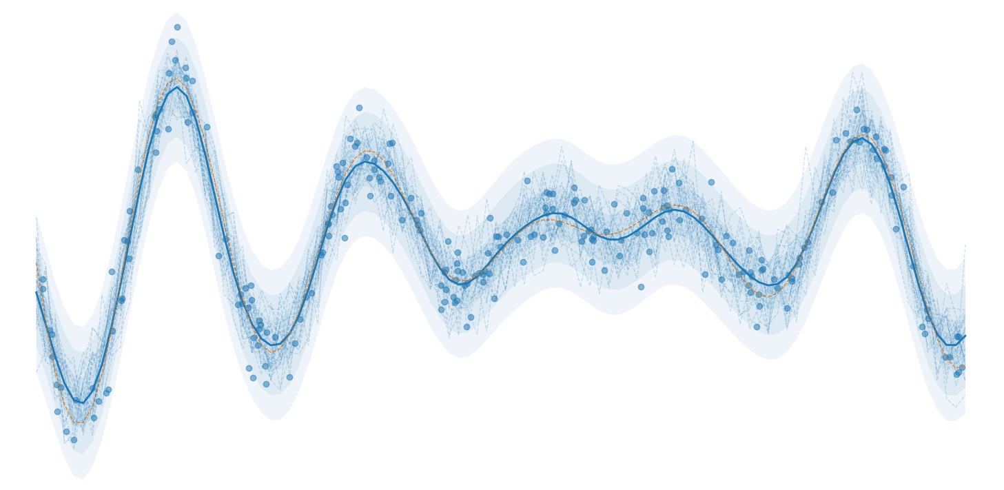
Matrix samples = model.getSamples(sampleCount);The artificial observation data and corresponding predictions/samples are saved in the observations.csv and predictions.csv/samples.csv files, respectively. The trained model results can be plotted using the provided Python script Plot.py.
For the two dimensional case (i.e. when inputDim=2 in the main.cpp file), an additional figure illustrating the predictive uncertainty of the model is provided; this plot corresponds to a slice of the predictive mean, transparent standard deviation bounds, and the observation data points used for training:
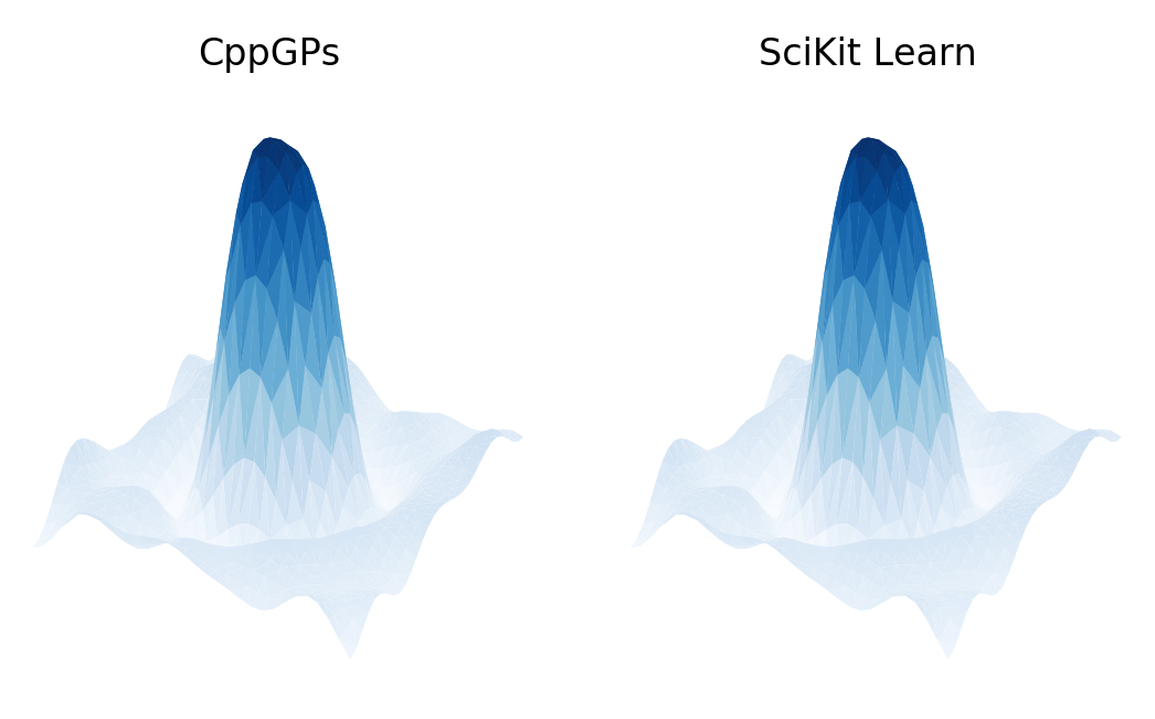
The results of the CppGP code and SciKit Learn GaussianProcessRegressor class can be compared using the Comparison_with_SciKit_Learn.py Python script. This code provides the estimated kernel/noise parameters and corresponding negative log marginal likelihood (NLML) calculations using the SciKit Learn framework. A qualitative comparison of the CppGP and SciKit Learn results can be plotted using the Plot_Comparisons.py script:
The VERIFY_NLML variable can also be set to True to validate the negative log marginal likelihood calculation computed by CppGP using the SciKit Learn framework.
The CppGP results can also be compared with two GPyTorch implementations of Gaussian processes: the standard GP model as well as a structured kernel interpolation (SKI) implementation. These results can be computed using the Comparison_with_GPyTorch.py script and can be plotted using the Plot_Comparisons.py script after setting the USE_GPyTorch variable to True.
The profiling steps below will not work with the current multi-threaded implementation. They have been included for reference, since these results provided the original motivation for incorporating multi-threading into certain parts of the current code.
valgrind- debugging/profiling tool suiteperf- performance analyzing tool for Linuxgraphviz- open source graph visualization softwaregprof2dot- python script for converting profiler output to dot graphs
Profiling data is produced via the callgrind tool in the valgrind suite:
valgrind --tool=callgrind --trace-children=yes ./Run
Note: This will take much more time to run than the standard execution time (e.g. 100x).
A graph visualization of the node-wise executation times in the program can then be created via:
perf record -g -- ./Run
perf script | c++filt | gprof2dot -s -n 5.25 -f perf | dot -Tpng -o misc/profilier_output.png
Note: The -s flag can also be removed from the gprof2dot call to show parameter types. The -n flag is used to specify the percentage threshold for ommitting nodes.
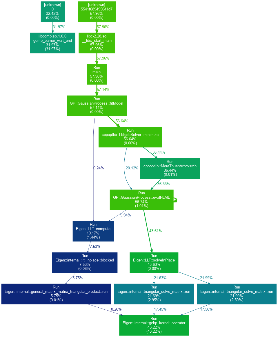
An example graph generated using the procedures outlined above is provided below:
As can be seen from the figure, the majority of the computational demand of the CppGP implementation results from the Eigen::LLT::solveInPlace method. This corresponds to the term cholesky.solve(Matrix::Identity(n,n)) in the evalNLML() function definition, which is used to compute the gradients of the NLML with respect to the hyperparameters. A simple multi-threaded implementation of this calculation has been incorporated into the code to achieve a considerable speed-up in the execution time.
Gaussian Processes for Machine Learning is an extremely useful reference written by Carl Rasmussen and Christopher Williams; the book has also been made freely available on the book webpage.
Eigen provides a header-only library for linear algebra, matrix operations, and solving linear systems. The Getting Started page of the Eigen documentation provides a basic introduction to the library.
LBFGS++ is a header-only C++ implementation of the limited-memory BFGS algorithm (L-BFGS) for unconstrained minimization written by Yixuan Qiu. It is based off of the libLBFGS C library developed by Naoaki Okazaki and also includes a detailed API.
CppOptimizationLibrary is an extensive header-only library written by Patrick Wieschollek with C++ implementations for a diverse collection of optimization algorithms; the library is availble in the GitHub repository PatWie/CppNumericalSolvers.
SciKit Learn provides a Gaussian Process Python module with an extensive collection of covariance kernels and options.


