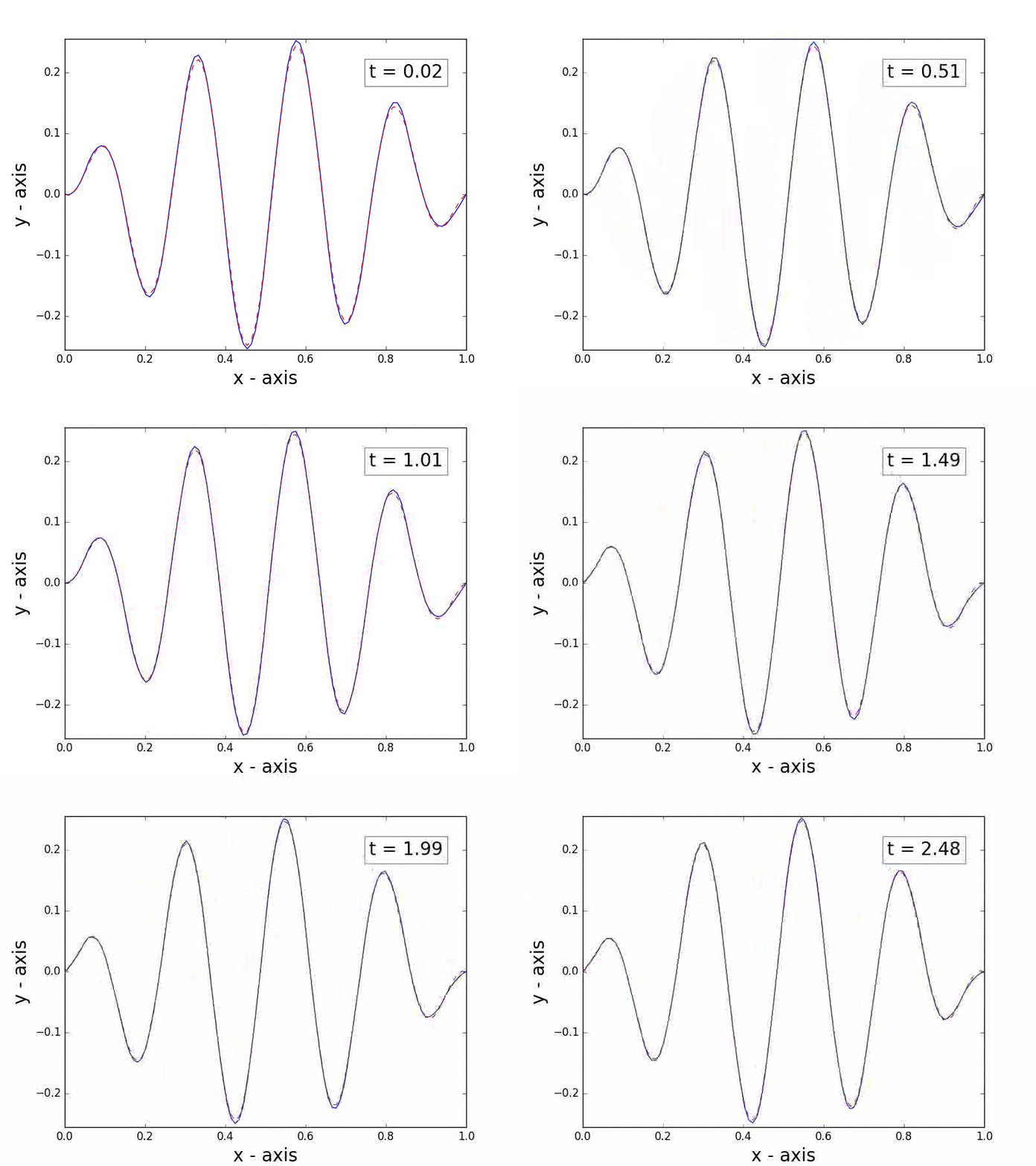
This code provides a simple, pedagogical implementation of the finite element method for solving parabolic partial differential equations (PDEs) in one dimension.
This code is designed to illustrate a collection of fundamental methods/techniques for solving PDEs using the finite element method. It is recommended that a more high-performance computing platform such as FEniCS is used for real applications of the finite element method. Setting up and solving partial differential equations in FEniCS is extremely straight-forward and much more numerically stable than the more pedagogical code provided in this repository.
The finite element space basis functions which are implemented in this code are:
linear_basis- linear basis functionsquadratic_basis- quadratic basis functions
The desired set of basis functions can be specified by setting the basis variable in the model.py file.
There are also two choices of solver methods available:
Cholesky- Solve using a Cholesky factorization and triangular inversionConjugate Gradient- Solve using the conjugate gradient method
which can specified by the solve_method variable.
Moreover, there are two time-stepping schemes:
Backward Euler- The implicit backward Euler schemeCrank-Nicolson- The Crank-Nicolson / Theta=0.5 scheme
which can be specified by the time_stepping variable.
The code can be run by simply issuing the command:
user@host $ python model.py

-------------------------
 Finite Element Space:  |
-------------------------

  - Spatial Domain = [0.00, 1.00]
  - Time Interval = [0.00, 0.15]
  - FEM Basis = Linear Basis Functions
  - Time Stepping = Crank-Nicolson
  - Solve Method = Conjugate Gradient
  - Problem Dimension = 99


-------------------------
 FEM Solver Progress:   |
-------------------------

  [ Forming Stiffness Matrix ]


  [ Forming Mass Matrix ]


  [ Computing Preconditioner ]


  [ Solving Linear System ]  (Step 101 of 101)


   Solve Time:  44.92097 seconds


  [ Saving Animation ]
This code will also generate and save an animation for the computed solution:
